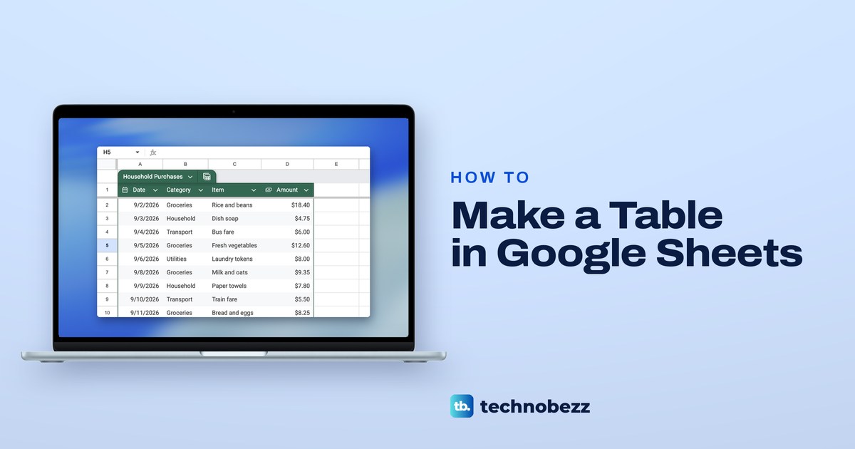
To make a table in Google Sheets, select your list together with its heading row, then choose Format > Convert to table. Sheets turns the range into a named table straight away, with a menu arrow on every heading, shaded rows and a frozen heading row. From there you can set a type for each column, add a total row and filter the rows without touching the data.
We turned a 12-row purchases list into a table in Chrome, named it, set its column types and added a total. One result surprised us: the table's own total ignores a filter, so it can show a figure that does not match the rows on screen.
The short version
- Convert a list: select it with its headings, then choose Format > Convert to table, or press Command + Option + T on a Mac and Ctrl + Alt + T on Windows.
- Name it: click the arrow beside the table's name and choose Rename table.
- Set column types: click the arrow in a heading and choose Edit column type, for example Currency or Dropdown.
- Add a total row: in the table menu, choose Table formatting > Show table footer.
- No data yet: choose Insert > Pre-built tables and pick Blank table or a ready-made one.
- Going back: Revert to unformatted data keeps your entries, while Delete table removes them.
Ways to make a table at a glance
| Method | Start from | What you get |
|---|---|---|
| Format > Convert to table | Your list, selected with its headings | A named table with column types, a table menu and views |
| On a Mac: Command + Option + T. On Windows: Ctrl + Alt + T. On ChromeOS: Shift + Alt + T. | The same selection | The same table, without opening the menu |
| Insert > Pre-built tables | An empty part of the sheet | A panel of ready-made tables, such as Blank table and Project tasks |
| Format > Alternating colors | Your list, selected | A colored heading row and banded rows, with no table features |
| The Google Sheets app | Cells selected with the blue markers | Fill color and borders from the Format button, which give the look of a table |
How to convert your data to a table
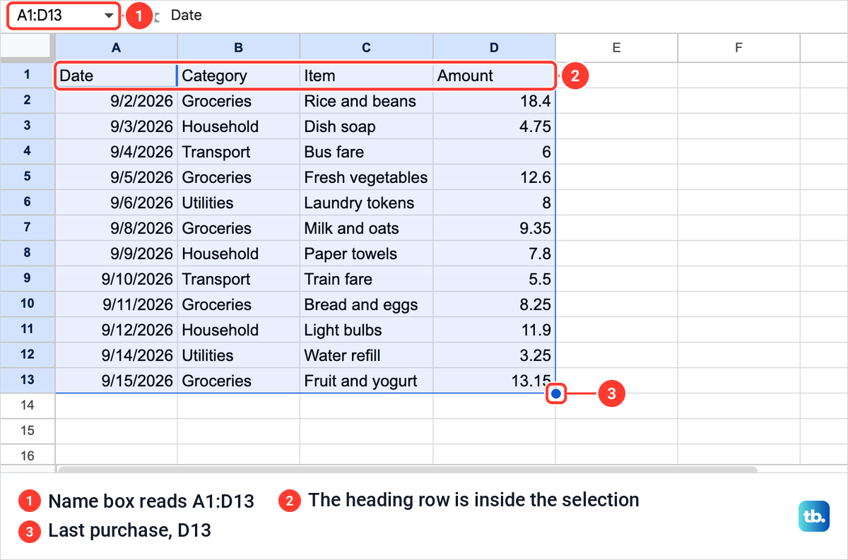
Start with a list that has one row of headings at the top and one record on each row below it. Ours, in a file called Home Spending, had the headings Date, Category, Item and Amount and 12 purchases under them. If the same entry appears twice, it is easier to remove duplicates in Google Sheets before the list becomes a table.
Click the first heading, hold Shift and click the last cell of the list, so the heading row is part of the selection. We selected A1 to D13, and the Name box at the left of the formula bar read A1:D13.
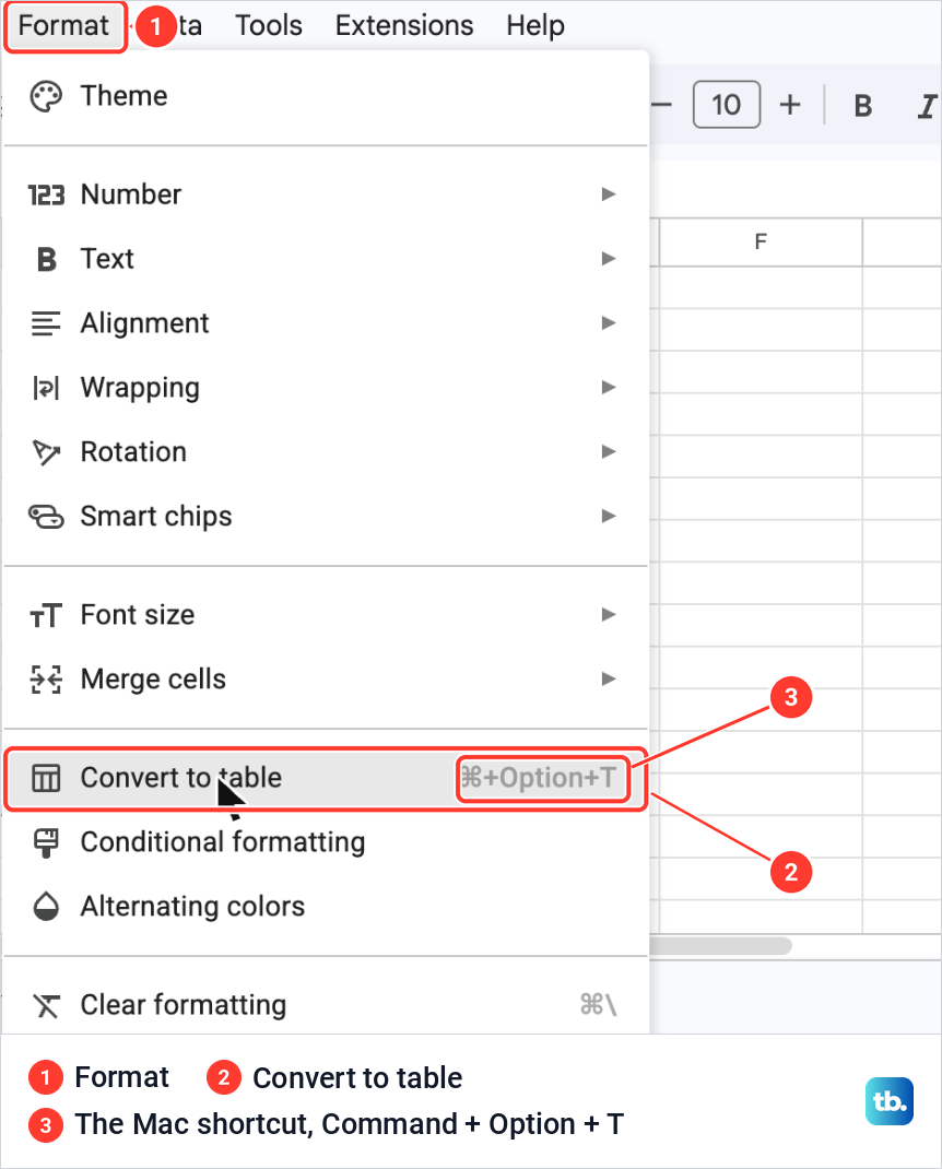
Now open the Format menu and choose Convert to table. On our Mac the menu printed the shortcut beside it, Command + Option + T. On Windows the same shortcut is Ctrl + Alt + T, and on ChromeOS it is Shift + Alt + T.
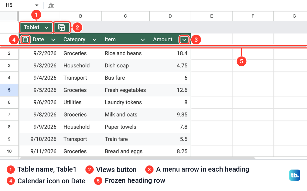
Sheets converted the range at once, with no dialog to fill in. A dark green tab above the list carried the name Table1, the headings turned dark green with a small arrow beside each one, and every second row was shaded. The values themselves did not change.
Two more things happened by themselves. The Date heading got a calendar icon, because Sheets gave that column the Date type, and the heading row was frozen, so it stays in view as you scroll. In an ordinary sheet you would do that with the steps to freeze a row in Google Sheets.
A tip card titled Change column type popped up over the rows the first time, with a note about setting column types such as dates and dropdowns. We closed it with its X.
Rename the table
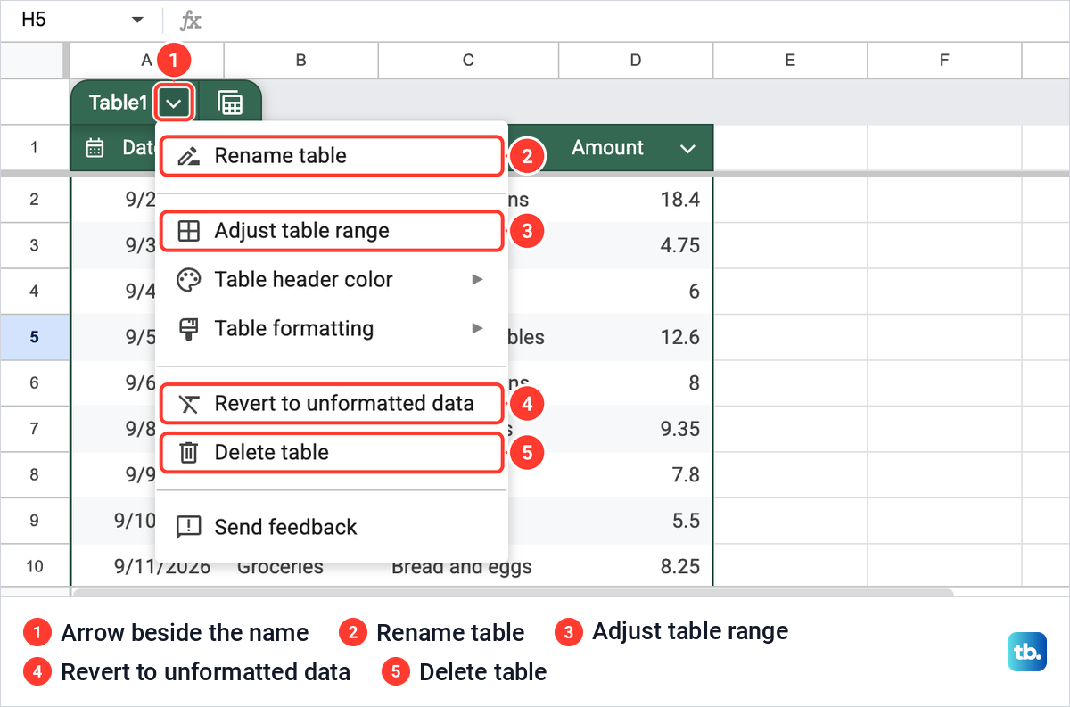
Every new table starts with a plain name such as Table1, and a clear name pays off once formulas use it. Click the small arrow beside the name to open the table menu. It holds Rename table, Adjust table range, Table header color, Table formatting, Revert to unformatted data and Delete table.
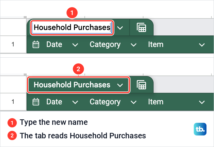
Choose Rename table, and the name turns into a text box. We typed Household Purchases and pressed Enter, and the tab kept the space between the two words. In formulas, Sheets writes that space as an underscore, as the total row further down shows.
A table name cannot start with a number, run past 255 characters, be TRUE or FALSE, or look like a cell address such as A1. Letters, numbers, spaces and underscores are all fine.
Set a type for each column
A column type tells Sheets what kind of entry belongs in a column. Click the arrow in a heading and point to Edit column type. The list offers Number, Text, Date, Dropdown, Checkbox, Smart chips and None, and Number opens a second list with Number, Percent and Currency.
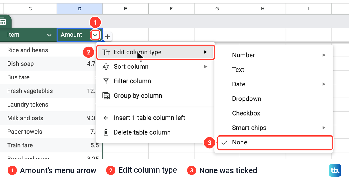
The same heading menu has Sort column, Filter column, Group by column, Insert 1 table column left and Delete table column. Our guide to sorting and alphabetizing in Google Sheets explains the sort orders, and for a sheet without a table there is our guide to adding columns in Google Sheets.
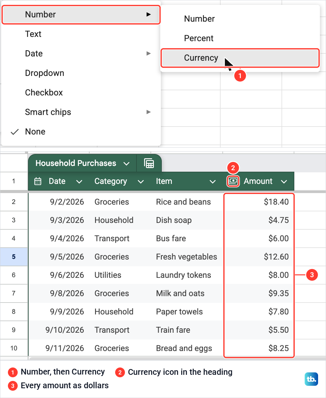
Our Amount column had None ticked, so its amounts were still plain numbers such as 18.4 and 6. We chose Number > Currency, and every amount changed to dollars with two decimals, such as $18.40 and $3.25. A small currency icon appeared in the heading.
A column type also keeps an eye on later entries. Sheets shows a warning on any cell in the column that does not follow its type, for example a word typed into a Currency column. For a column that has to hold mixed entries, choose None.
Turn a column into a drop-down list
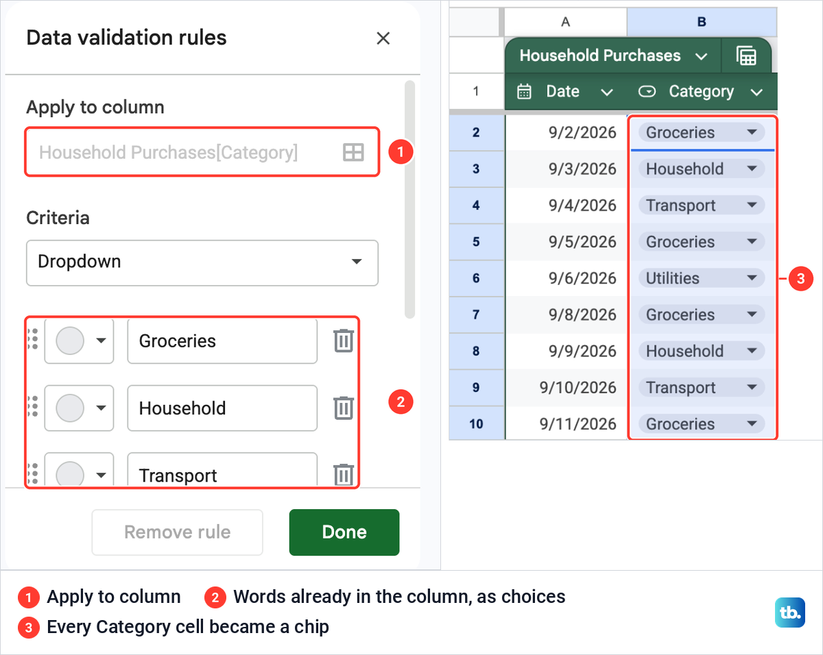
Dropdown is the type to use for a column of set words such as categories. We chose it for Category, and a panel named Data validation rules opened on the right. Its Apply to column box read Household Purchases[Category], and the four words already in the column, Groceries, Household, Transport and Utilities, were filled in as the choices.
Every Category cell turned into a chip with an arrow, and a note at the bottom of the screen read Table column type updated to dropdown list. Clicking a chip opened the four choices, with a pencil at the bottom for editing the list. Click Done to close the panel.
Our guide to creating a drop-down list in Google Sheets covers lists outside a table, including what happens when someone types a word that is not on the list. For a done or not done column, choose the Checkbox type instead, and our guide to adding checkboxes in Google Sheets explains what a ticked box stores.
Add a total row to the table
Open the table menu again, point to Table formatting and choose Show table footer. The same submenu has Show table gridlines, Show alternating colors, which was ticked by default, Show condensed view and View advanced options.
A shaded row appeared under the last purchase, and under Amount it showed $108.95, the total of all 12 amounts. When we clicked that cell, the formula bar read =SUM(Household_Purchases[Amount]). Sheets wrote that formula itself, naming the table and the column instead of a range of cells, with an underscore where our table name has a space.
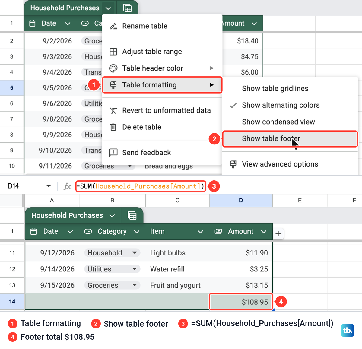
Because the formula names the column rather than fixed cells, it kept up when we added a row, as the next section shows. Outside a table, our guide to totaling a column in Google Sheets covers the plain SUM route. With the total in place, you can make a graph in Google Sheets from the same columns.
Add rows to a table
To add a purchase in the middle of the table, right-click one of its rows. The menu speaks in table terms, with Insert 1 table row above, Insert 1 table column left, Delete table row and Delete table column. For blocks of rows in a sheet without a table, our guide to inserting multiple rows in Google Sheets covers the row-number route.
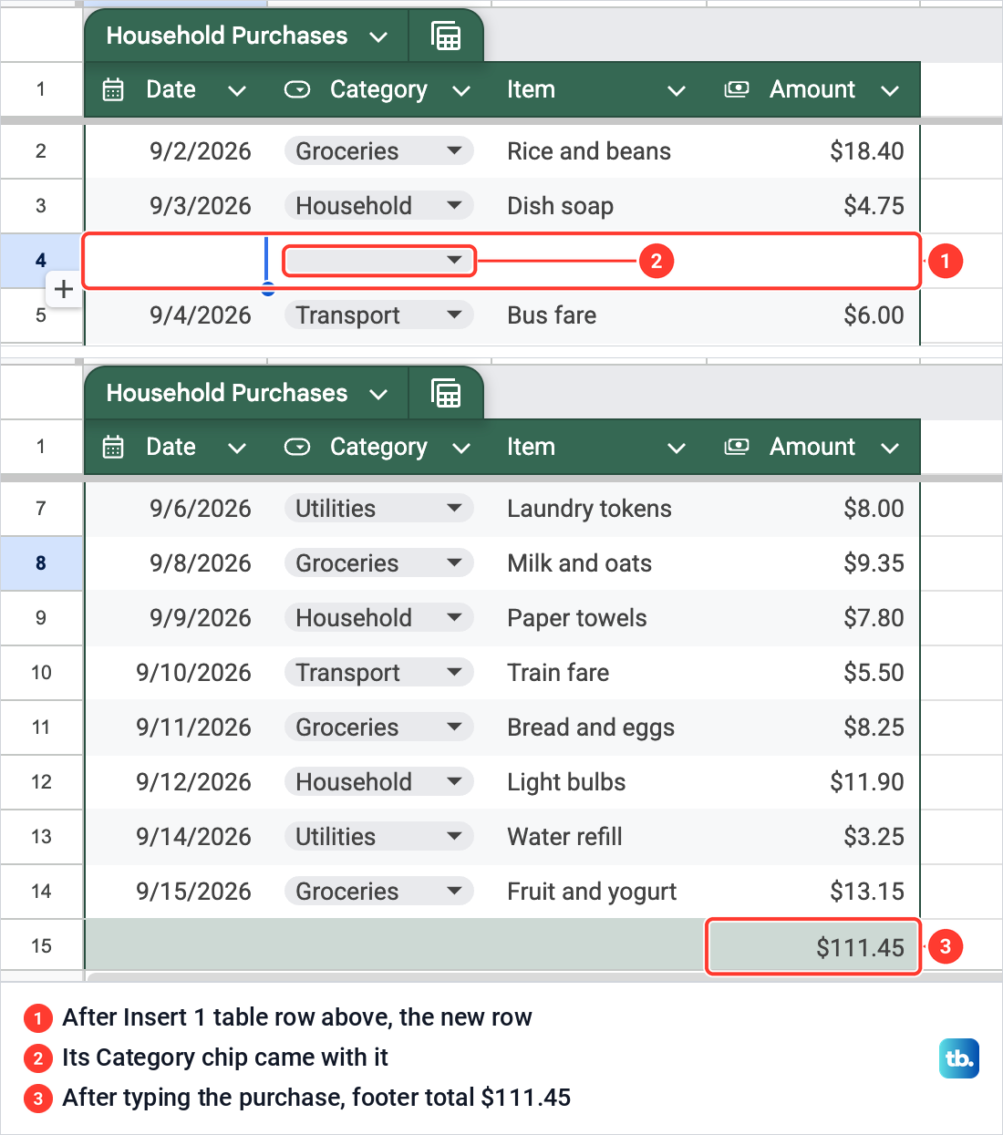
We chose Insert 1 table row above, and an empty row appeared inside the table as row 4, with an empty Category chip already in it. Then we typed a purchase into it: 9/3/2026, Household, Sponges and 2.5. The amount took the currency format by itself, and the footer total rose from $108.95 to $111.45.
Pressing Command + Z five times took the row and its entries away again. On Windows and ChromeOS, undo is Ctrl + Z.
With the footer showing, the date we typed in the first row below it stayed outside the table, an ordinary cell with the total unchanged. Pressing Tab in the last cell of the last row also moved out of the table without adding a row, so add new rows from inside the table.
Group and filter a table without changing it for others
The button with a grid icon beside the table name holds views. It offers Create group by view, with a list of the table's columns, and Create filter view. A view changes what you see, not what other people with the file see.
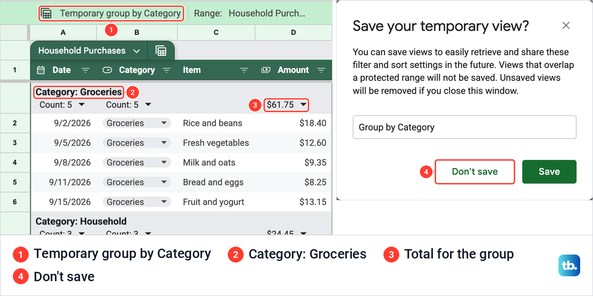
We grouped by Category. A green bar at the top read Temporary group by Category, and the rows sat under headings such as Category: Groceries, with a count of 5 and the group's total, $61.75.
Closing the view with the X at the right end of the green bar asked Save your temporary view?, with Don't save and Save. We chose Don't save, and the table went back to its normal order. A view you do not save also disappears when the spreadsheet refreshes, and saving one needs edit access to the file.
A filter view starts the same way. We chose Create filter view, the bar read Temporary filter 1, and the arrows in the headings became filter buttons. In the Category list we clicked Clear, ticked Groceries only and clicked OK.
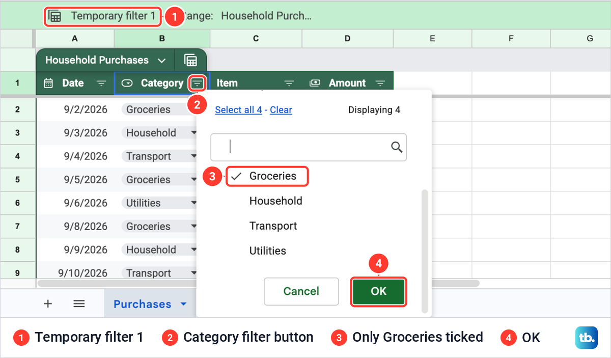
Five rows were left, and the status bar read 6 of 13 rows displayed, a count that includes the heading row. The footer still read $108.95, the total of all twelve purchases, not the $61.75 that the five Groceries rows add up to.
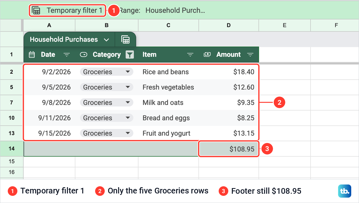
So read the footer as the total of the whole table, whatever is on screen. For the total of one category, the group by view above gives it directly. We closed the filter view with Don't save as well.
Start with a pre-built table
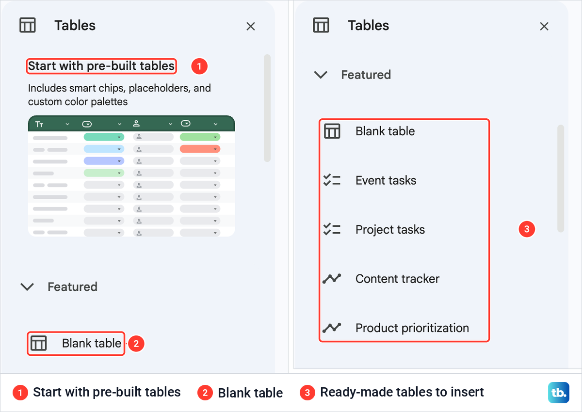
If you have no data yet, choose Insert > Pre-built tables. A panel named Tables opened on the right, headed Start with pre-built tables, with the note Includes smart chips, placeholders, and custom color palettes.
Under Featured it listed Blank table, Event tasks, Project tasks, Content tracker, Product prioritization and Recruitment applicants. Blank table is the one for your own headings, and the others arrive with their columns already laid out.
An empty range works too. Select some empty cells, choose Format > Convert to table, and type your headings into the new table.
Make a simple table without the table features
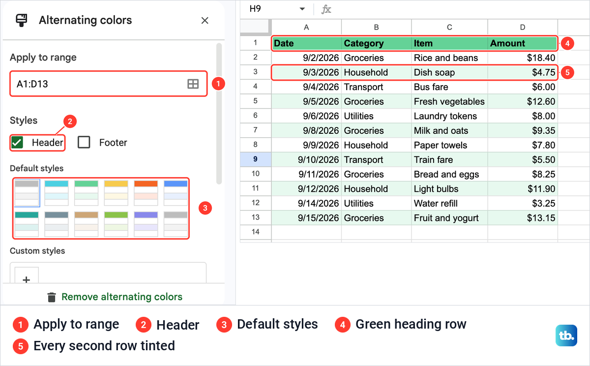
Sometimes a list only needs to look tidy, for example before you print it. Select the range, choose Format > Alternating colors and pick a style. We did this on a plain copy of the same list, with the headings in bold.
The panel showed Apply to range A1:D13, a Header box that was ticked, a Footer box, twelve default styles and a Custom styles area. After we picked the green style, the heading row turned green and every second row was tinted. There was no name tab, no arrow in the headings and no table menu, so the list was still an ordinary range.
To finish the look, the toolbar above the sheet has buttons for bold, cell fill color and borders, and long entries sit better once you wrap text in Google Sheets. A styled range like this can still become a real table later with Format > Convert to table.
Turn a table back into a normal range
The table menu has two ways out, and they are not the same. Revert to unformatted data removes the table's style and leaves every entry where it is. Delete table removes the table and its data.
Use Revert to unformatted data when you want your plain list back. Keep Delete table for a table you no longer need at all, entries included.
When a table does not behave as expected
If the table covers the wrong rows, open the table menu and choose Adjust table range. Ours opened a box named Select a data range holding Purchases!A1:D14, which shows that the footer row counts as part of the range. Type the range you want and click OK, or click Cancel to leave it as it is.
In our table, a date typed under the footer stayed outside the table, as we saw above. Insert new rows from inside the table, or widen the range here to take in rows that are already typed.
A warning on a cell in a typed column usually means the entry is the wrong kind, such as text in a Currency column. Retype it, or set the column's type to None. If a total looks wrong, check whether a filter view is open, because the footer counts hidden rows too.
Format cells like a table on Android, iPhone or iPad
In the Google Sheets app, you give cells the look of a table with the Format button. On an Android phone or tablet, open the spreadsheet, tap a cell and drag the blue markers across the cells you want. Tap Format and open the Cell tab, which has Cell fill color, Alternating colors and Borders.
Use the Text tab of the same panel for bold headings, then tap the sheet to save your changes. On an iPhone or iPad the steps are the same, but the Cell tab lists Cell fill color, Borders, Wrap text and Merge cells, so fill every second row yourself if you want bands.
How we tested this guide
We tested this in Google Sheets on the web in Chrome on a Mac, converting a 12-row purchases list to a table and setting its column types, footer total and views.
Frequently Asked Questions
Where is Convert to table in Google Sheets?
It is in the Format menu. Select your list with its heading row, then choose Format > Convert to table, or press Command + Option + T on a Mac, Ctrl + Alt + T on Windows or Shift + Alt + T on ChromeOS.
Can I turn empty cells into a table?
Yes. Select the empty cells and choose Format > Convert to table, then type your headings. Insert > Pre-built tables also offers Blank table and ready-made tables such as Event tasks.
Does Delete table keep my data?
No. Delete table removes the table and the entries in it. To keep your entries and drop only the table's style, choose Revert to unformatted data in the table menu instead.
Why doesn't the table's total change when I filter it?
The footer total counts every row in the table. In our table it stayed at $108.95 with only the five Groceries rows on screen. For one category's total, use a group by view, which showed $61.75 for Groceries.
How do I use a table name in a formula?
Write the table name with the column name in square brackets, such as =SUM(Household_Purchases[Amount]), the formula Sheets wrote for our footer. A space in the table name becomes an underscore in the formula.
Can I make a table in the Google Sheets app?
Convert to table is in the Format menu of Google Sheets on a computer. In the app, you can give cells the look of a table: select them with the blue markers, tap Format and use the Cell tab for fill color and borders, and on Android also for alternating colors.
Is a range with colors and borders the same as a table?
No. A styled range only changes how the cells look. A table also has a name, a type for each column, a table menu, views and a total row that follows rows you insert inside the table.