To wrap text in Google Sheets, select the cells, then choose Format > Wrapping > Wrap. Long entries then run onto extra lines inside their own cells, and the row grows taller to show them unless it has been given a set height. On a phone, tap Format and choose Wrap text in the Cell tab.
We wrapped a column of long notes in our home tasks sheet and ran into two things the menu does not explain. The Wrapping submenu showed no mark on the setting in use, and a row with a set height kept hiding the extra lines. Both are covered below.
The short version
- One cell or a range: select it, then choose Format > Wrapping > Wrap.
- A whole column: click its letter first. For the whole sheet, click the empty box above row 1.
- From the toolbar: the Text wrapping button offers Overflow, Wrap and Clip and highlights the one in use.
- Lines still hidden: right-click the row number, choose Resize row, then Fit to data.
- A new line inside one cell: press Command + Enter on a Mac or Ctrl + Enter on Windows while you type.
- On a phone: tap Format, open the Cell tab and choose Wrap text.
How to wrap text in a cell
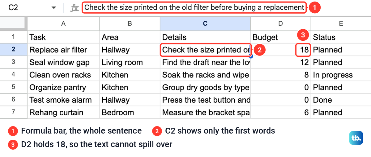
Cells start on Overflow by default, which keeps text on one line. In our sheet, the Details sentences stopped at the edge of column D, because the Budget cells beside them hold numbers. When we selected C2, the formula bar above the grid showed the whole sentence, while the cell itself showed only its opening words.
To wrap it, click the cell, or drag across several cells to select a range. Open the Format menu at the top, point to Wrapping, which sits between Alignment and Rotation, and choose Wrap. The submenu lists three choices, Overflow, Wrap and Clip.
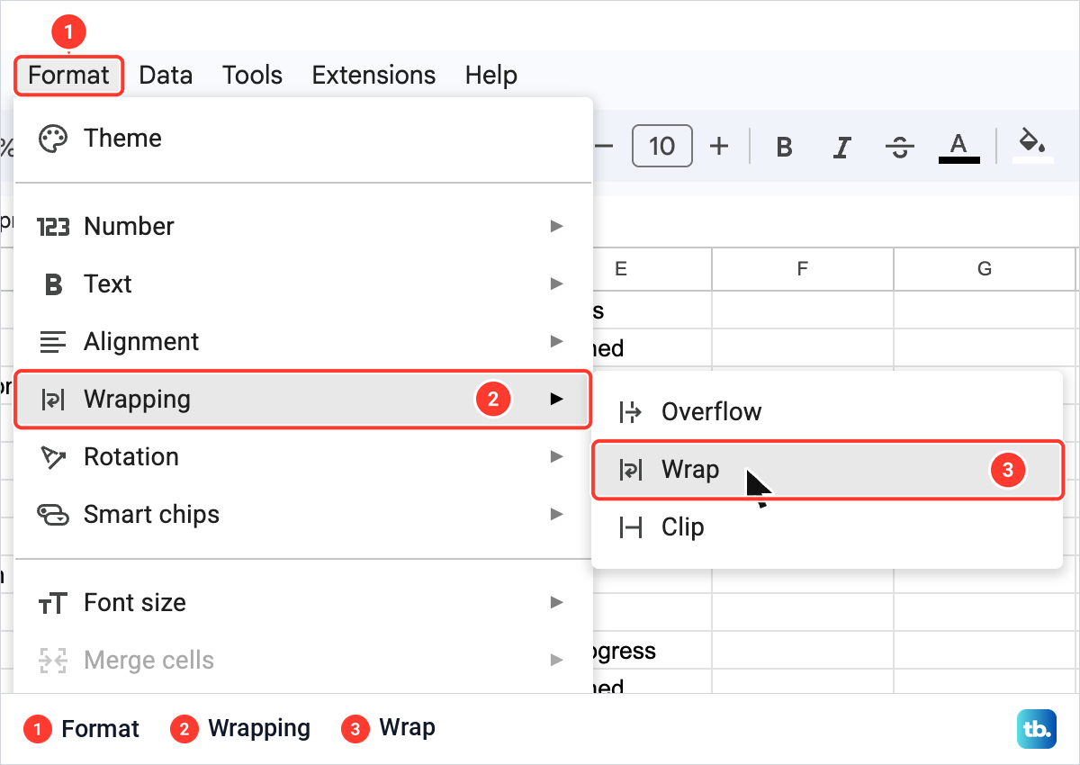
The submenu does not tell you which one is in use. When we opened it on a cell that was still on the default, none of the three had a tick or any other mark. The toolbar button in the next section does show the current setting.
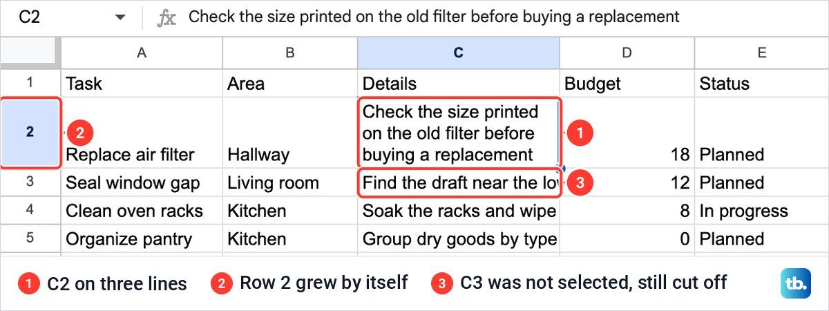
After we chose Wrap, the sentence in C2 sat on three lines inside the cell and row 2 grew taller by itself. The task name, budget and status in that row moved to the bottom of the taller row. Rows 3 to 15 did not change, because only C2 was selected.
Wrap text from the toolbar
The Text wrapping button on the toolbar is the quicker route. In our window it sat between the vertical align and text rotation buttons, just left of the three-dot More button. Click it and three icons drop down, which read Overflow, Wrap and Clip from left to right when you rest the pointer on them.
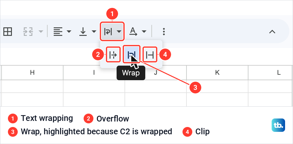
Unlike the Format menu, this button marks the setting in use. With the wrapped C2 selected, the middle icon, Wrap, was highlighted in blue, so this is the place to check what a cell is set to. If you do not see the button, Format > Wrapping > Wrap does the same job.
How to wrap a whole column or the whole sheet
To wrap a whole column, click its letter at the top of the grid. The Name box at the left of the formula bar then reads C:C for column C. Choose Format > Wrapping > Wrap and every cell in that column wraps at once.
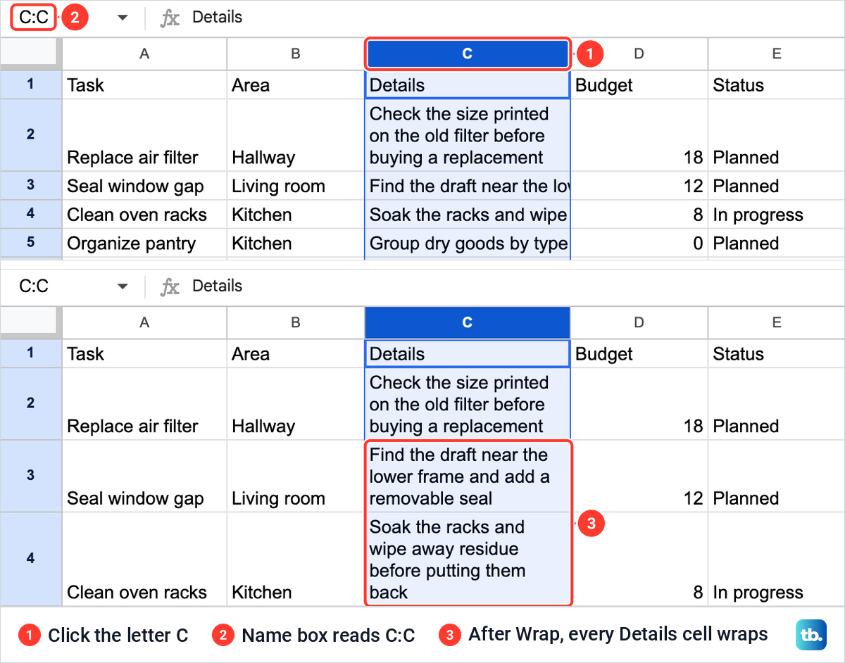
In our sheet, each Details note went onto three or four lines and every row grew to fit, so rows 2 to 6 filled the screen. Taller rows push the headings out of view sooner as you scroll. To keep the headings in view, freeze a row in Google Sheets.
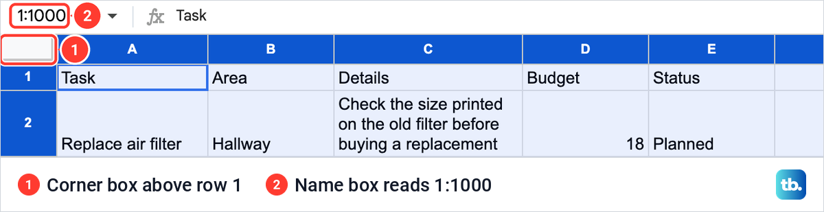
To wrap everything, click the empty box above row 1 and to the left of column A. That selects the whole sheet: the Name box read 1:1000 in our sheet, and every column letter and row number turned blue. Then choose Wrap from the Format menu or the toolbar as before.
What Overflow, Wrap and Clip do
The three settings only change how the text is shown. The whole entry stays in the cell either way, and the formula bar showed the full sentence under every setting we tried.
| Setting | What the cell shows | When the next cell holds something | Best for |
|---|---|---|---|
| Overflow, the default | One line that runs on into empty neighboring cells | The text stops at the edge of its own cell | Short notes beside empty columns |
| Wrap | Extra lines inside the cell, and the row grows unless it has a set height | No change, the text stays inside its cell | Reading full notes in a narrow column |
| Clip | One line, cut at the cell's own right edge | No change, it is cut either way | Showing one line of text per cell |
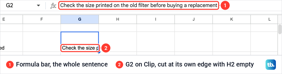
To compare them, we typed the C2 sentence into G2. On Overflow, it ran across the empty cells to its right as far as column J. As soon as we typed Note into H2, G2 showed only "Check the size p" and stopped at the edge of its own cell.
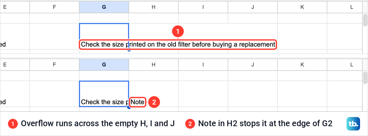
Clip cut the same sentence at G2's own right edge, even with H2 empty again. Click the cell and the formula bar still shows every word, so nothing is deleted.
Why some wrapped text is still hidden
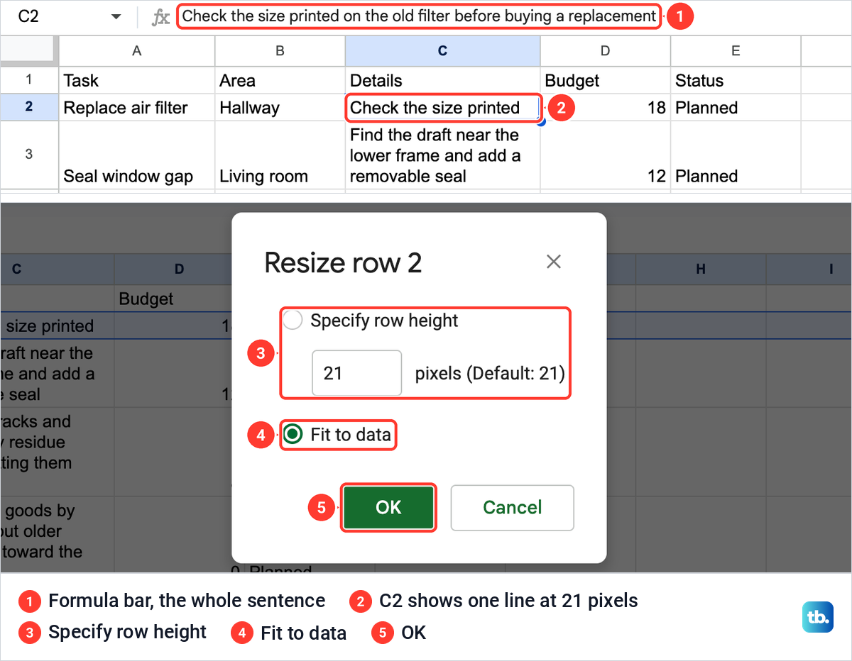
If a wrapped cell still shows one line, the row has probably been given a set height. We set row 2 to 21 pixels with Resize row, and C2 went back to showing only "Check the size printed", although it was still set to Wrap.
To fix it, right-click the row number and choose Resize row. A box titled Resize row 2 opened with two choices, Specify row height with a pixels field and Fit to data. Select Fit to data, then OK, and every wrapped line comes back.
A double-click works too. With the row at 21 pixels again, we double-clicked the lower border of row 2 in the row numbers on the left, and the row fitted itself to the three lines. To fix many rows at once, select their row numbers first, then right-click any one of them.
Make the column wider to keep rows short
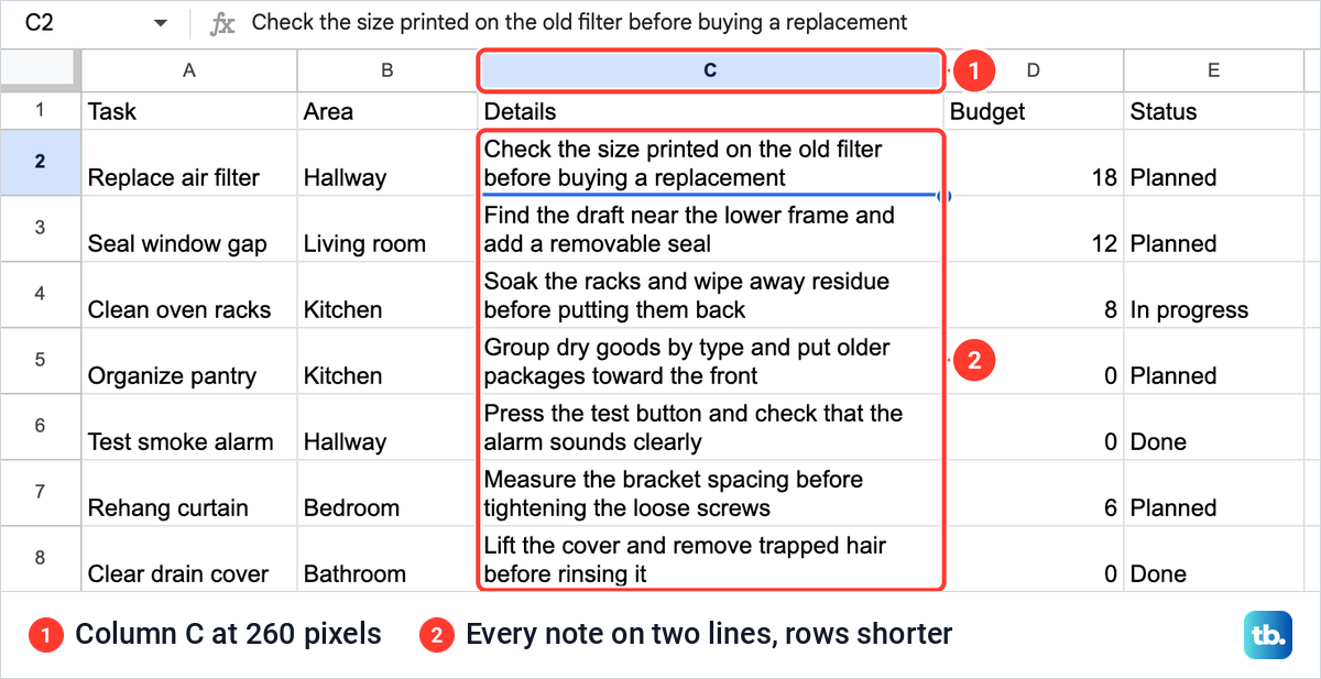
A narrow wrapped column makes tall rows, so the width is your other control. Right-click the column letter and choose Resize column. The Resize column C box asks you to enter a new column width in pixels, shows the default of 100 and offers Fit to data as well. You can also drag the border on the right of the column letter.
Width changes the number of lines, not whether the text wraps. At 150 pixels, our Details notes took three or four lines each. At 260 pixels every note took two lines, and the rows shrank by themselves without another Fit to data.
How to start a new line inside a cell
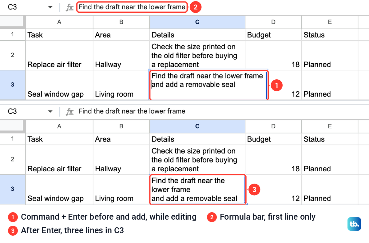
Wrap breaks lines wherever the column edge happens to fall. To start a new line at a word you choose, double-click the cell, click where the new line should begin, and press Command + Enter on a Mac or Ctrl + Enter on Windows. Press Enter on its own when you are done.
With column C set back to 170 pixels, we put the cursor before "and add" in C3 and pressed Command + Enter. While we were still editing, the cell showed two lines, and after Enter it showed three, the break we added plus one where the wrap met the column edge. The one-line formula bar showed only the first line, "Find the draft near the lower frame".
On a phone, double-tap the cell to edit it, then touch and hold the text. On Android, choose Insert line break or press Ctrl + Enter on a keyboard, and on an iPhone or iPad choose Next > Insert line break or press Command + Enter. Tap Done when you finish.
How to wrap text on Android, iPhone and iPad
In the Google Sheets app on Android, tap a cell, then drag the blue markers across any nearby cells you want. Tap Format, open the Cell tab and choose Wrap text, then tap the sheet to save the change.
The steps on an iPhone or iPad are the same. Tap a cell, drag the blue markers to take in more cells if you need them, then tap Format and choose Wrap text in the Cell tab. Tap the sheet when you are done.
Check wrapped text before you print
Wrapped lines carry over to the print preview just as they look on screen. We chose File > Print, which is Command + P on a Mac or Ctrl + P on Windows, and Sheets opened its own Print settings page. The preview showed the Details column with every wrapped line, including the break we added in row 3.
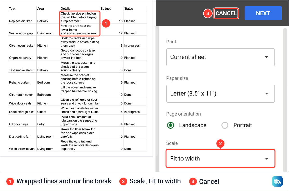
In the panel beside the preview, Scale was on Fit to width, and all five of our columns fitted across the page. Choose Next to go on to Chrome's print window, or Cancel to go back to the sheet.
A tall wrapped table can run over several pages. To repeat the heading row on each page, freeze it, then open Headers & footers in Print settings and choose Repeat frozen rows.
If you choose Next and your printer shows as offline, follow our steps to fix a printer that shows offline. To show someone the table without printing it, you can take a screenshot on a Mac or take a screenshot on Windows.
Once every note is readable, the table is easier to work with. You can alphabetize and sort in Google Sheets by any column, remove duplicates in Google Sheets if a task was entered twice, or select the data with its headings and make a graph in Google Sheets from the Budget figures.
How we tested this guide
We tested this in Google Sheets on the web in Chrome on a Mac, wrapping, clipping and resizing a column of long notes in a 14-row home tasks sheet.
Frequently Asked Questions
Why is my wrapped text still cut off?
The row most likely has a set height. Right-click the row number, choose Resize row, select Fit to data and click OK, or double-click the row's lower border. If the text is not wrapped at all, the Text wrapping button on the toolbar shows which setting the cell is on.
Can I wrap an entire column?
Yes. Click the column letter to select the whole column, then choose Format > Wrapping > Wrap. Every cell in the column wraps, and rows grow to fit unless they have a set height.
Is there a keyboard shortcut to wrap text in Google Sheets?
No single key wraps text in Sheets. You can open the Format menu from the keyboard with Alt + O in Chrome on Windows, Alt + Shift + O in other browsers or Ctrl + Option + O on a Mac, then choose Wrapping > Wrap. For a new line at a point you choose, press Command + Enter on a Mac or Ctrl + Enter on Windows while you edit the cell.
What is the difference between Wrap and Clip?
Wrap shows the whole entry on extra lines, and a row without a set height grows to fit. Clip shows only one line of text, cut at the cell's right edge, even when the next cell is empty. Either way, the full entry stays in the cell.
How do I unwrap text in Google Sheets?
Select the cells and choose Format > Wrapping > Overflow, the default, or Clip if you want each entry cut at the cell edge. If a row stays taller than you want, right-click its number, choose Resize row and enter a height.