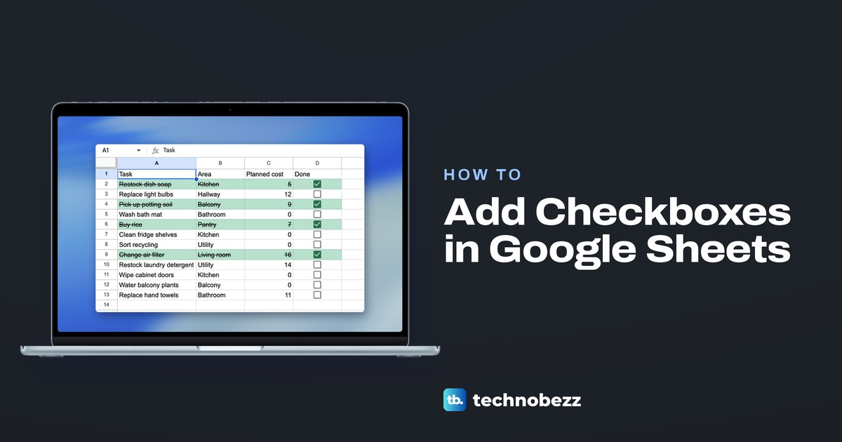
To add check boxes in Google Sheets, select the cells, then choose Insert > Checkbox. Every selected cell gets an empty box that holds FALSE by default, and a click ticks it and turns the value to TRUE. In the Android app, select the cells and tap More > Data validation > Checkbox. On an iPhone or iPad, add the boxes on a computer first and tick them in the app.
We turned a 12-task errands list into a Google Sheets checklist, then counted, filtered and colored its rows by the boxes. Two results are worth knowing before you start. Pressing Delete on a box, ticked or not, removed the box itself, so that cell dropped out of the count, and switching the boxes to your own words breaks every formula and color rule that looked for TRUE or FALSE until you change those too.
The short version
- Add boxes: select empty cells, such as a Done column under its heading, then choose Insert > Checkbox.
- Tick several at once: select them and press Space. A click ticks a single box.
- Count the ticks: =COUNTIF(D2:D13,TRUE) counts the ticked boxes in D2 to D13.
- Remove boxes: select them and press Delete. An empty cell is not FALSE, so your counts change.
- Your own words: open Data > Data validation, click the Checkbox rule and tick Use custom cell values, then change any formula that looks for TRUE or FALSE.
- On a phone: on Android, tap More > Data validation > Checkbox. On an iPhone or iPad, add the boxes on a computer.
Checkbox tasks at a glance
The cell references below match our errands list, with its boxes in D2 to D13. Change them to fit your own sheet.
| Task | How to do it | What to expect |
|---|---|---|
| Add boxes on a computer | Select the cells, then Insert > Checkbox | An empty box in every selected cell, FALSE by default |
| Tick one box or several | Click a box, or select several and press Space | A ticked box holds TRUE by default |
| Count ticked boxes | =COUNTIF(D2:D13,TRUE) in an empty cell | 4 for the four tasks we ticked |
| Remove boxes | Select them and press Delete | An empty cell, which no longer counts as FALSE |
| Copy a box to a new row | Command + C and Command + V on a Mac, Ctrl + C and Ctrl + V on Windows | A working box in the new cell |
| Add boxes on Android | Select the cells, tap More > Data validation, then Checkbox | Boxes added in the Sheets app |
| Use boxes on iPhone or iPad | Add them on a computer, then open the sheet in the app | Check and uncheck existing boxes |
How to add checkboxes in Google Sheets
Pick an empty column for the boxes, beside the items you want to tick off. Our errands list had Task, Area and Planned cost in columns A to C, and a Done heading in D1 with nothing below it. Select the cells under the heading only, either by dragging down the column or by typing the range, such as D2:D13, into the Name box at the left of the formula bar and pressing Enter.
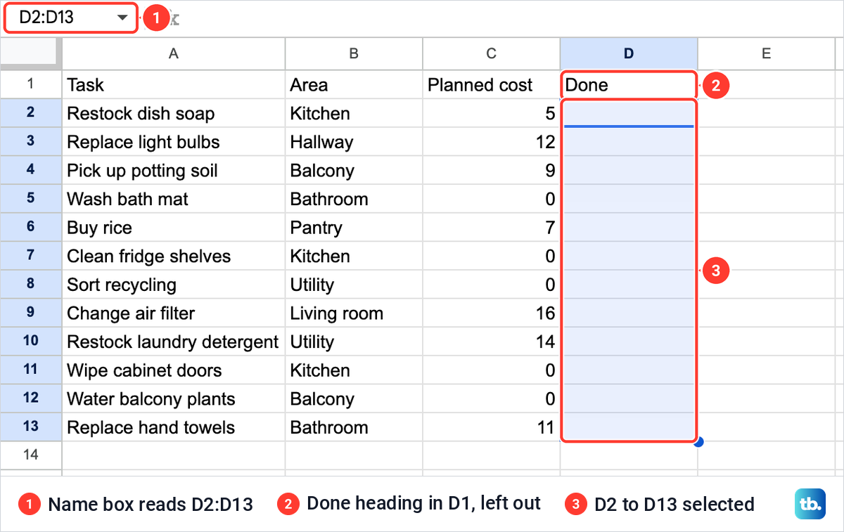
Leave the heading out of the selection, so only the cells you will tick get a box. If your list has no free column yet, add one beside the tasks first. Twelve tasks fit on one screen, but on a longer list you can freeze a row in Google Sheets so the Done heading stays in view while you work down the column.
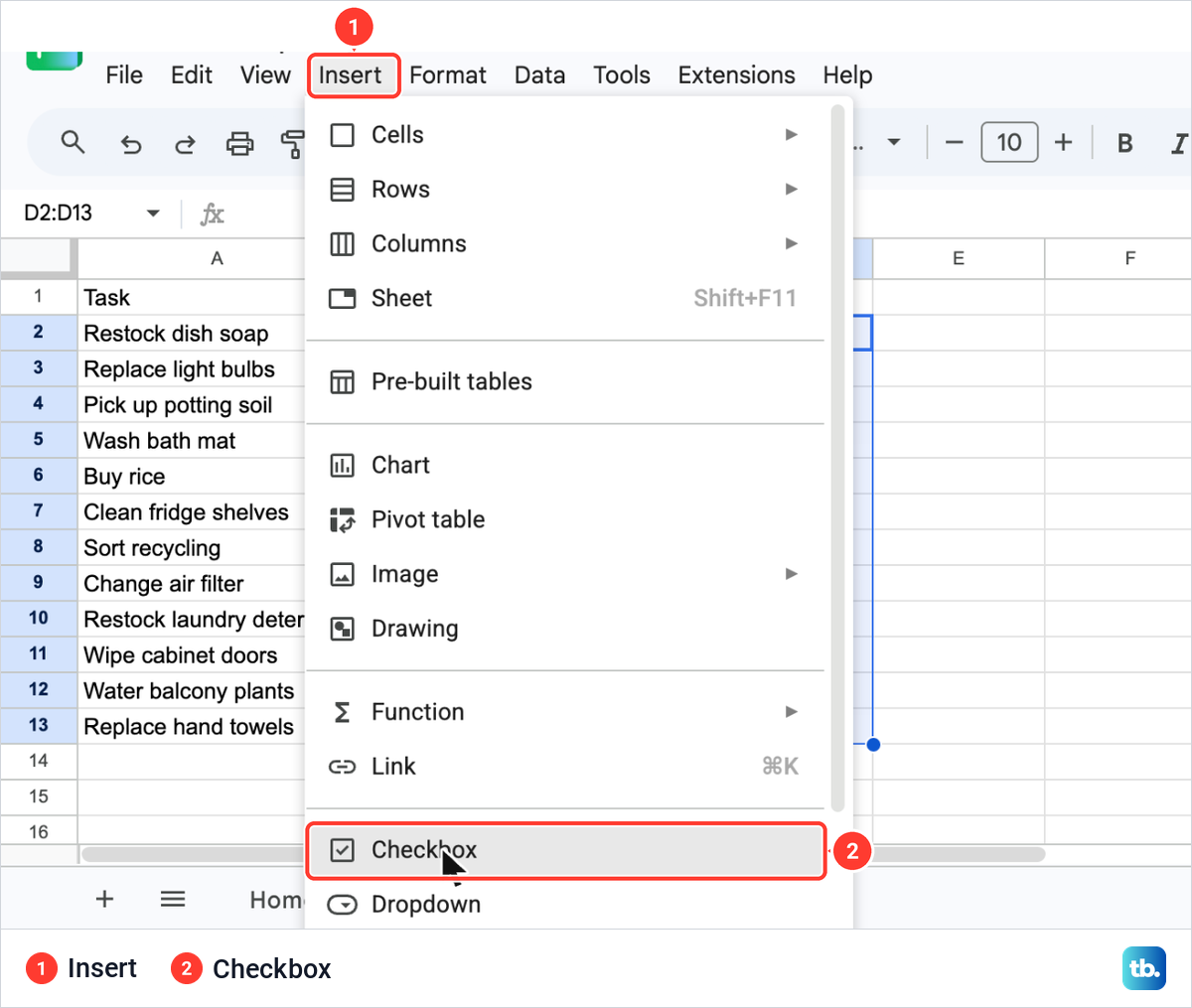
With the cells selected, open the Insert menu at the top and choose Checkbox. In our menu it sat near the bottom, below Function and Link and just above Dropdown, the entry you use to create a drop-down list in Google Sheets.
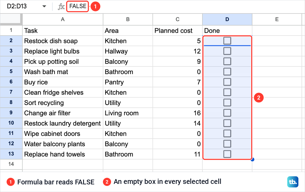
Every selected cell got an empty box at once, centered in the cell. With D2 to D13 still selected, the formula bar read FALSE, the value an unticked box holds by default. From here the column works like any other data, so you can count it, filter it and color rows by it.
If your task names run past the edge of their column, wrap the text or widen the column so each task shows in full beside its box. A long name is cut off at the edge of its cell whenever the next cell holds something, and in our list the Area column sits right beside the task names.
Tick a box and read its value
Click a box to tick it, and click it again to clear it. We ticked the boxes for Restock dish soap, Pick up potting soil, Buy rice and Change air filter, in D2, D4, D6 and D9. Each ticked box turned dark grey with a white tick.
The formula bar shows what the cell holds. With D2 selected it read TRUE, and with the unticked D3 selected it read FALSE. Those two words are the defaults, and every count, filter and color rule in this guide works with them.
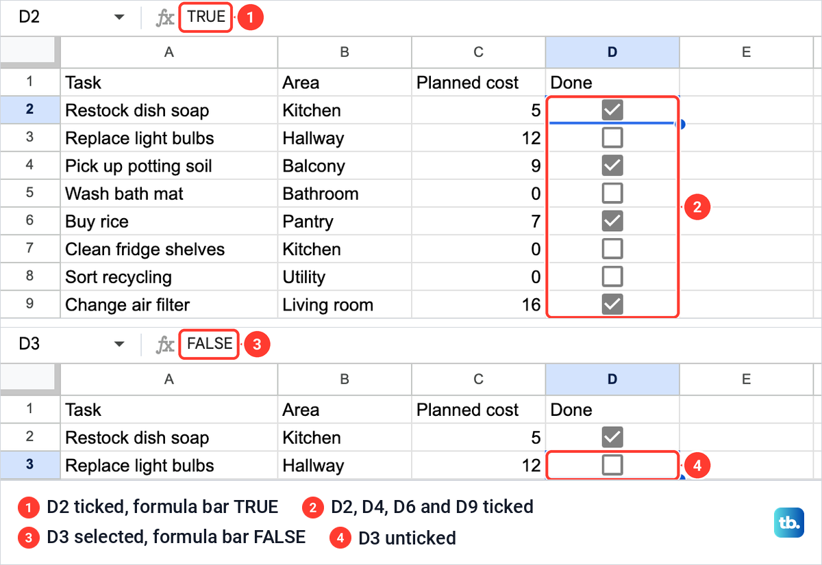
To change many boxes at once, select them and press Space. We selected D2 to D5, two ticked and two empty, and one press ticked all four rather than flipping each box, while a second press cleared all four. On our Mac, Command + Z pressed twice put the original mix back. On Windows or ChromeOS, undo is Ctrl + Z.
Count checked boxes with COUNTIF
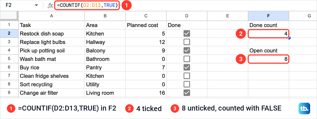
Because a ticked box holds TRUE, a COUNTIF formula can count the ticks. Click an empty cell beside the table, type the formula with your own range and press Enter. We put a Done count label in F1 and this formula in F2.
=COUNTIF(D2:D13,TRUE)It returned 4, one for each ticked task. For the tasks still open, change TRUE to FALSE. Our =COUNTIF(D2:D13,FALSE) in F5, under an Open count label, returned 8, and the two counts add up to the 12 boxes in the column.
If the same task sits in two rows and both boxes are ticked, the count includes both. Check the list for repeated tasks before you rely on the number, and remove duplicates in Google Sheets once you are sure they are true repeats. Checkboxes also work with charts, so you can make a graph in Google Sheets from the two counts.
Remove a checkbox without deleting the task
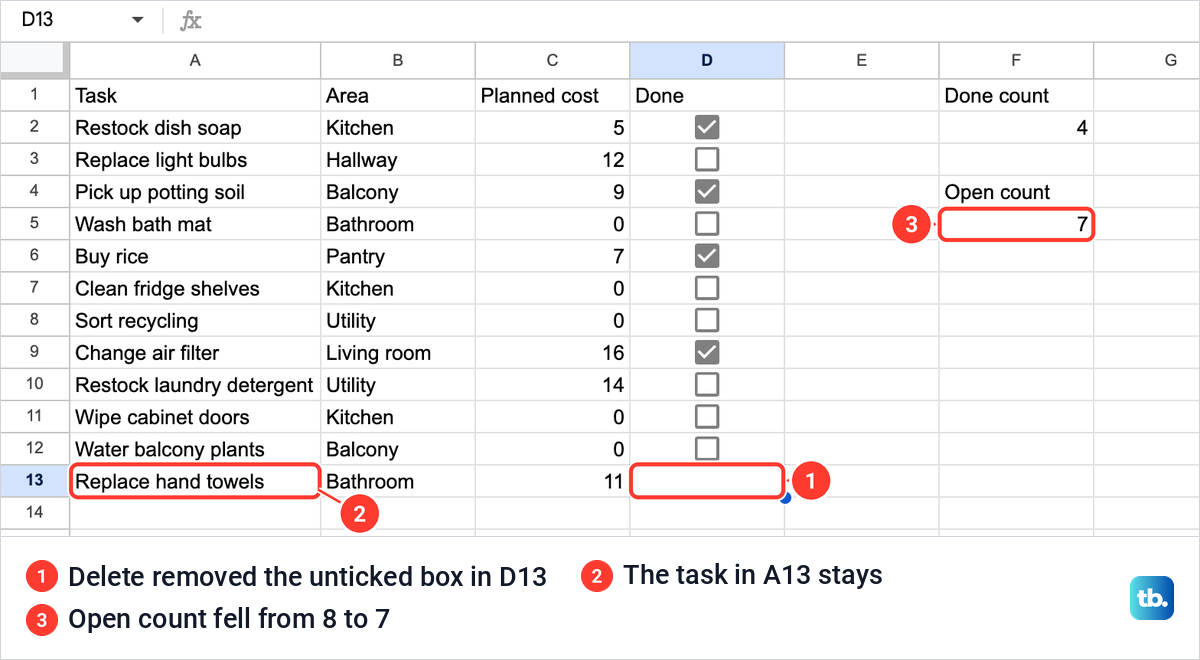
Unticking a box and removing it are different things. To remove a box, select its cell and press Delete. When we did that on the unticked D13, the box disappeared and the cell went empty, while Replace hand towels stayed in A13 and the rest of the row was untouched.
The count changed too. An empty cell is not FALSE, so our Open count fell from 8 to 7 although nobody had ticked anything. A ticked box went the same way: Delete removed it and the count of finished tasks fell from 4 to 3.
If a count drops after a cleanup, look for cells in the column that lost their box. Command + Z brought the box back on our Mac, and Ctrl + Z does the same on Windows and ChromeOS.
To clear the boxes from a whole column, select all of them, press Delete and check that the cells are empty. To give a new task a box instead, copy an existing box into the new row, after you insert rows in Google Sheets if the task belongs in the middle of the list.
We copied the unticked D13 with Command + C and pasted it into D14 with Command + V, and D14 held a working box that read FALSE. On Windows and ChromeOS, use Ctrl + C and Ctrl + V.
A box below the end of your range sits outside formulas such as =COUNTIF(D2:D13,TRUE). Widen the range in each formula, to D2:D14 for one new row, so the new task is counted.
Show only the ticked tasks with a filter
A filter hides the rows you do not need without moving anything. Select the whole table with its headings, A1:D13 in our sheet, and choose Data > Create a filter. A filter button appears in each heading cell.
Click the button on the Done heading and open Filter by values. Our list showed just two entries, FALSE and TRUE, both ticked. Untick FALSE, click OK, and only the ticked tasks remain.
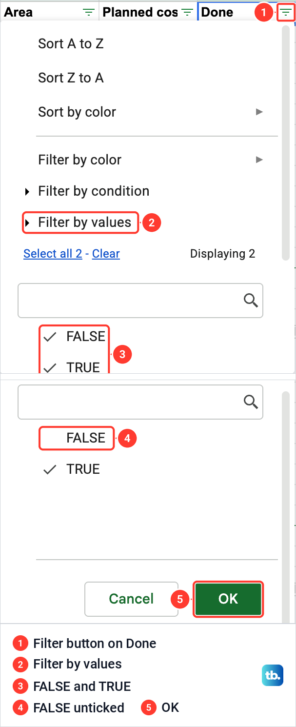
Our sheet then showed rows 2, 4, 6 and 9, the four ticked tasks, and the status bar read "4 of 12 rows displayed". The filter button on Done turned solid green to show that the column is filtered. Choose Data > Remove filter to bring every row back.
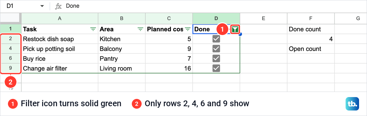
A filter changes the view for everyone who opens the file, and anyone who can edit it can change the filter. To reorder the list by the Done column instead of hiding rows, sort the whole table, never column D on its own, so each box stays beside its task. Our guide to alphabetize and sort in Google Sheets shows the safe way to do it.
Color a row when its box is ticked
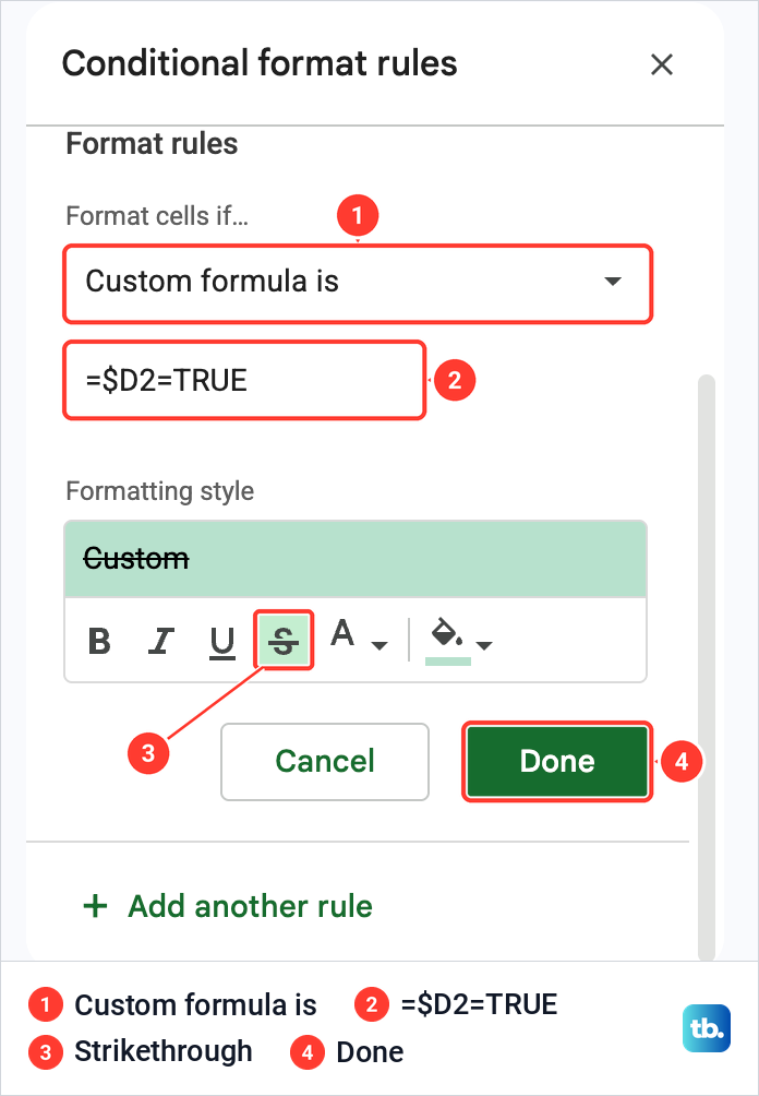
Conditional formatting can shade a task and strike it through as soon as its box is ticked. Select the table without its headings, A2:D13 in our sheet, and choose Format > Conditional formatting. In the panel, set Format cells if to Custom formula is and type the rule for the first row.
=$D2=TRUEThe dollar sign keeps every row looking at column D, while the 2 moves down one row at a time through the range. We kept the default pale green fill, turned on Strikethrough under Formatting style and clicked Done. The new look showed in the sheet before we clicked Done, which makes the rule easy to check.
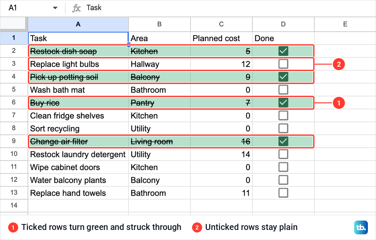
The four ticked rows turned pale green from A to D with every word struck through, and their boxes turned dark green. The eight unticked rows stayed plain. Any row whose box holds TRUE matches the rule, so the shading follows the ticks.
Use your own words instead of TRUE and FALSE
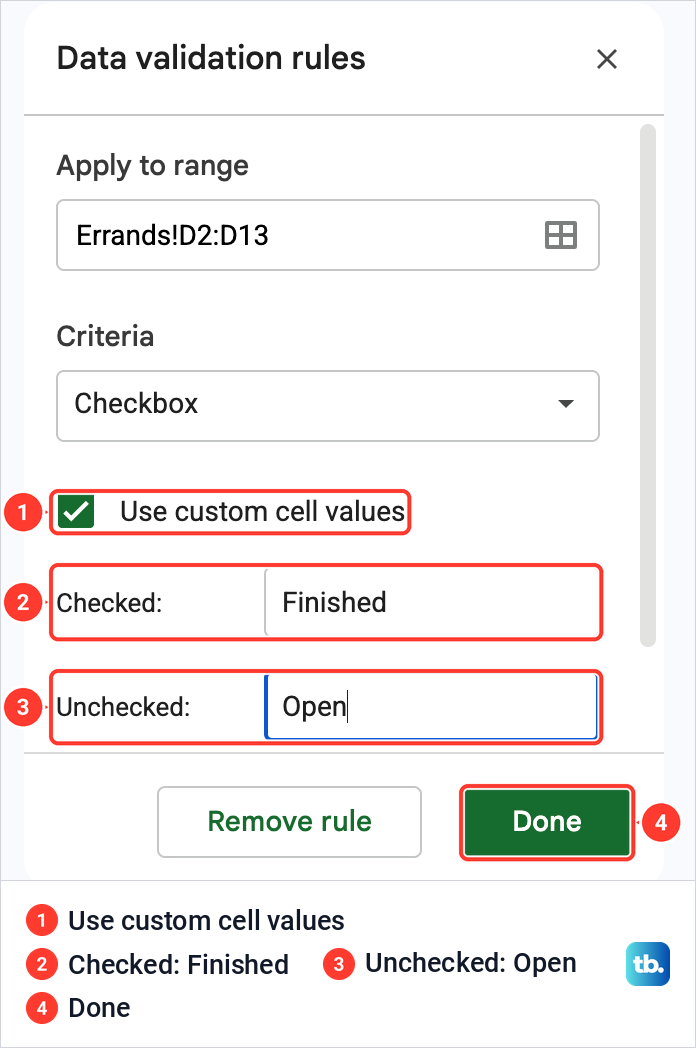
A checkbox is a data validation rule, and that rule is where its values are set. Select the boxes, D2:D13 in our sheet, and choose Data > Data validation. Our panel listed one rule, Checkbox, for D2:D13, and clicking it opened the rule with Criteria set to Checkbox and a tick box labelled Use custom cell values.
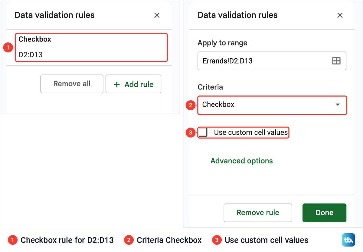
Tick Use custom cell values and two fields appear, Checked and Unchecked. We typed Finished for Checked and Open for Unchecked, then clicked Done. Only the Checked value is required.
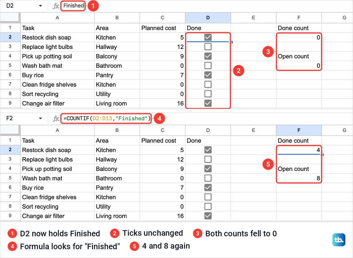
Here is the catch. The ticks stayed exactly where they were, but the cells now held the words, so D2 read Finished in the formula bar. Both COUNTIF formulas dropped to 0 at once, and the green, struck-through rows went plain, because nothing in the column equals TRUE or FALSE anymore.
Every formula that looked for the old values needs the new words, in quotes. We changed F2 to =COUNTIF(D2:D13,"Finished") and F5 to =COUNTIF(D2:D13,"Open"), and they returned 4 and 8 again. The color rule needs the same change, from =$D2=TRUE to =$D2="Finished", so open Format > Conditional formatting, click the rule and edit its formula.
Custom words suit a column that has to read as text, for a report or an export. If you switch, review the formulas, filter choices and color rules that look for TRUE or FALSE, and change them to your words at the same time. Leave the defaults alone when you do not need words.
Add checkboxes on Android, iPhone and iPad
The Google Sheets app for Android adds boxes through data validation. Open the spreadsheet in the app and select the cells you want to have checkboxes. Tap More at the top right, then Data validation, and in the list under Criteria tap Checkbox.
On an iPhone or iPad, add the boxes in Google Sheets on a computer first, as described above. Once they are in the sheet, you can check and uncheck them in the Sheets app on your iPhone or iPad.
How we tested this guide
We tested this in Google Sheets on the web in Chrome on a Mac, adding checkboxes to a 12-task errands list and then counting, filtering and coloring rows by them.
Frequently Asked Questions
Can I add checkboxes to many cells at once?
Yes. Select the whole range first, such as the empty cells under a Done heading, then choose Insert > Checkbox, and every selected cell gets its own box.
Can I add a checkbox in the Google Sheets app on iPhone?
Add the boxes in Google Sheets on a computer first. After that, you can check and uncheck them in the Sheets app on your iPhone or iPad.
What value does a checked box have in Google Sheets?
A ticked box holds TRUE by default and an empty one holds FALSE, which you can see in the formula bar. If the boxes use custom values, the cell holds your Checked or Unchecked word instead.
How do I count checked boxes in Google Sheets?
Use COUNTIF with the range of boxes and TRUE, such as =COUNTIF(D2:D13,TRUE), which returned 4 on our list. With custom values, put the Checked word in quotes, as in =COUNTIF(D2:D13,"Finished").
How do I remove checkboxes but keep my tasks?
Select only the cells with boxes, press Delete and check that the cells are empty. When we did this on an unticked box, the box went and the task text in the same row stayed.
Why can I see the boxes but not tick them?
You may only have view or comment access to the file, and viewers and commenters cannot make changes. Anyone who can edit the file can also protect a range so only some people can change it. That is set under Data > Protect sheets and ranges, so ask the owner whether your boxes are protected.