
To total a column in Google Sheets, click the empty cell under the numbers, type =SUM(D2:D13) with your own first and last cell, and press Enter. The total stays in that cell. For a quick look without a formula, select the numbers and read Sum in the box at the bottom right of the window.
We added up 12 purchases in our spending sheet, with the amounts in column D, and two results are worth knowing before you start. A whole-column formula, =SUM(D2:D), counted the ordinary total under the list as well and showed 217.9 instead of 108.95. And an amount stored as text was left out of both our totals without any warning.
The short version
- A total in a cell: click under the numbers, type =SUM(D2:D13) and press Enter.
- A quick look: select the numbers and read Sum at the bottom right. Nothing is saved.
- No typing: select the numbers, open the Functions button (the sigma, which may sit under More), choose SUM and press Enter.
- A list that grows: put =SUM(D2:D) in another column, never under the list.
- One category: use =SUMIF(B2:B13,"Groceries",D2:D13).
Ways to total a column at a glance
| What you want | What to do | Where the answer shows |
|---|---|---|
| A total that stays in the sheet | Type =SUM(D2:D13) under the list and press Enter | In that cell, here D14 |
| A quick look, nothing saved | Select D2:D13 | The Sum box at the bottom right of the window |
| SUM without typing | Select D2:D13, then Functions > SUM, then Enter | The first empty cell under the amounts |
| A total that takes new rows | Type =SUM(D2:D) in another column | Outside column D, here F2 |
| One category only | Type =SUMIF(B2:B13,"Groceries",D2:D13) | Any cell outside the range, here F2 |
| Only the rows a filter shows | Type =SUBTOTAL(9,D2:D13) | Any cell outside the range |
Every formula here uses our layout: headings in row 1, categories in column B and 12 amounts in D2:D13. Change the letters and row numbers to match your own sheet.
Add up a column with the SUM formula
Click the first empty cell under your numbers. In our sheet the amounts run from D2 to D13 under the heading Amount, so the total goes in D14.
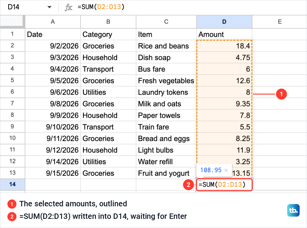
Type an equals sign, SUM and an opening parenthesis, then the first cell, a colon and the last cell. Start at the first amount, not at the heading. With =SUM(D2:D13 typed and no closing parenthesis yet, Sheets shaded the cells in the range, and a small box above the cell already showed the result, 108.95.
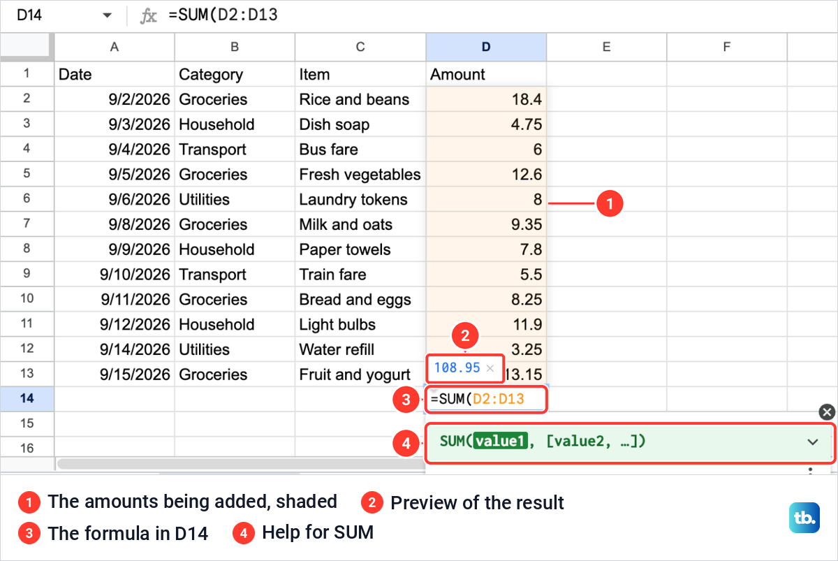
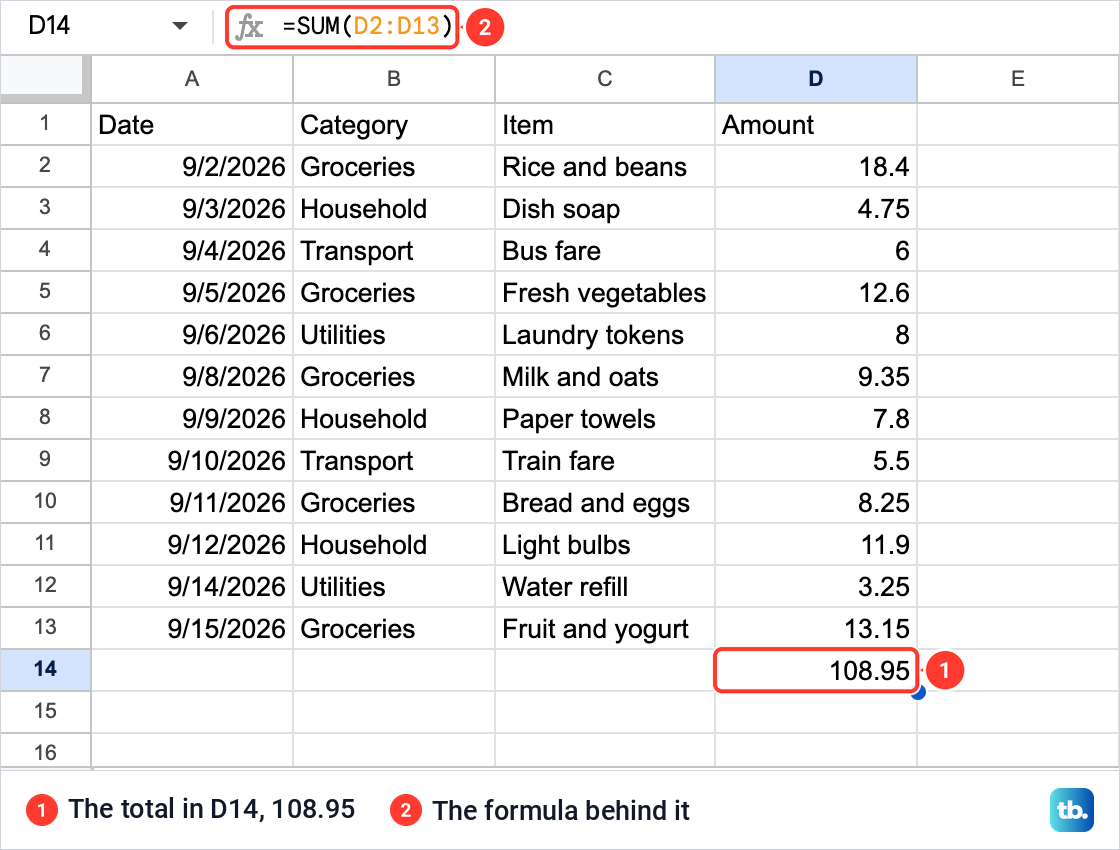
A help card for SUM opened under the cell as well, showing SUM(value1, [value2, ...]). Type the closing parenthesis and press Enter. D14 then showed 108.95, and with D14 selected, the formula bar above the sheet read =SUM(D2:D13).
You can also select the amounts with the mouse while the formula is open, instead of typing the range. The formula keeps working as you correct amounts, so there is nothing to redo after a fix.
See the total without a formula
For a quick answer you do not need to keep, select the numbers. We selected D2:D13, the Name box at the top left read D2:D13, and a green box at the bottom right of the window read Sum: 108.95.
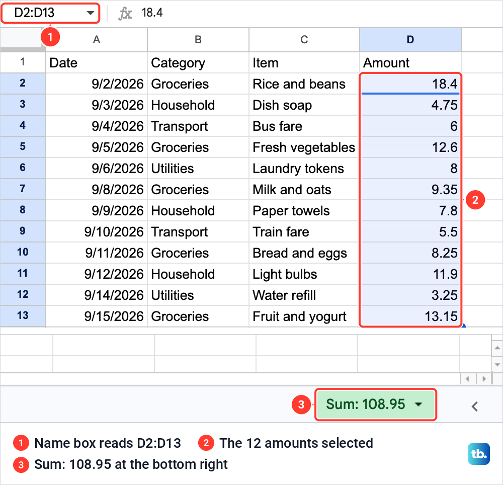
Nothing is written into the sheet, because the box only reads the cells you have selected. Leave an existing total out of the selection, or it is counted along with the amounts.
Click the box to see more. Ours listed Sum: 108.95, Avg: 9.079166667, Min: 3.25, Max: 18.4, Count: 12 and Count Numbers: 12. Choose one of them, such as Avg, to show it in the box instead of Sum.
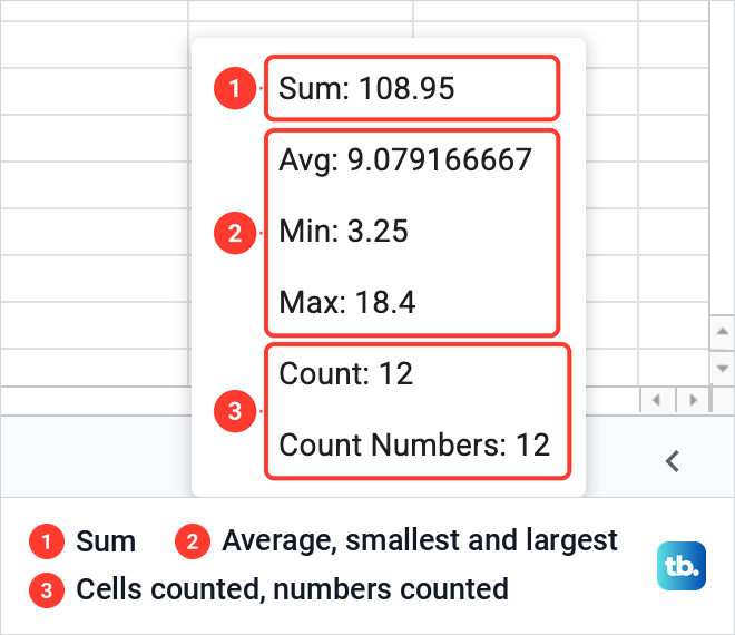
From the keyboard, Option + Shift + Q on a Mac, or Alt + Shift + Q on Windows and ChromeOS, moves to that list while cells are selected. The box does not work with some number and currency formats, so use the SUM formula when it shows no sum.
Use the Functions button
The toolbar has a Functions button, marked with the Greek letter sigma. In our window it was not on the toolbar itself but under the three-dot More button at the right end. Its list starts with SUM, AVERAGE, COUNT, MAX and MIN.
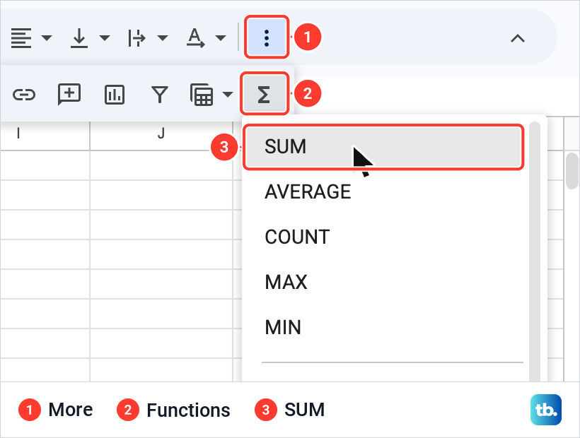
Select the amounts first. With D2:D13 selected, Functions > SUM wrote =SUM(D2:D13) into D14, the first empty cell under the selection. It outlined the range and waited for Enter.
With an empty cell selected instead, the button is far less helpful. The same choice wrote only =SUM( ) with no range at all, so you type or select the cells yourself. Either way, read the range before you press Enter, because the button adds exactly what was selected and nothing more.
Keep the total current as the list grows
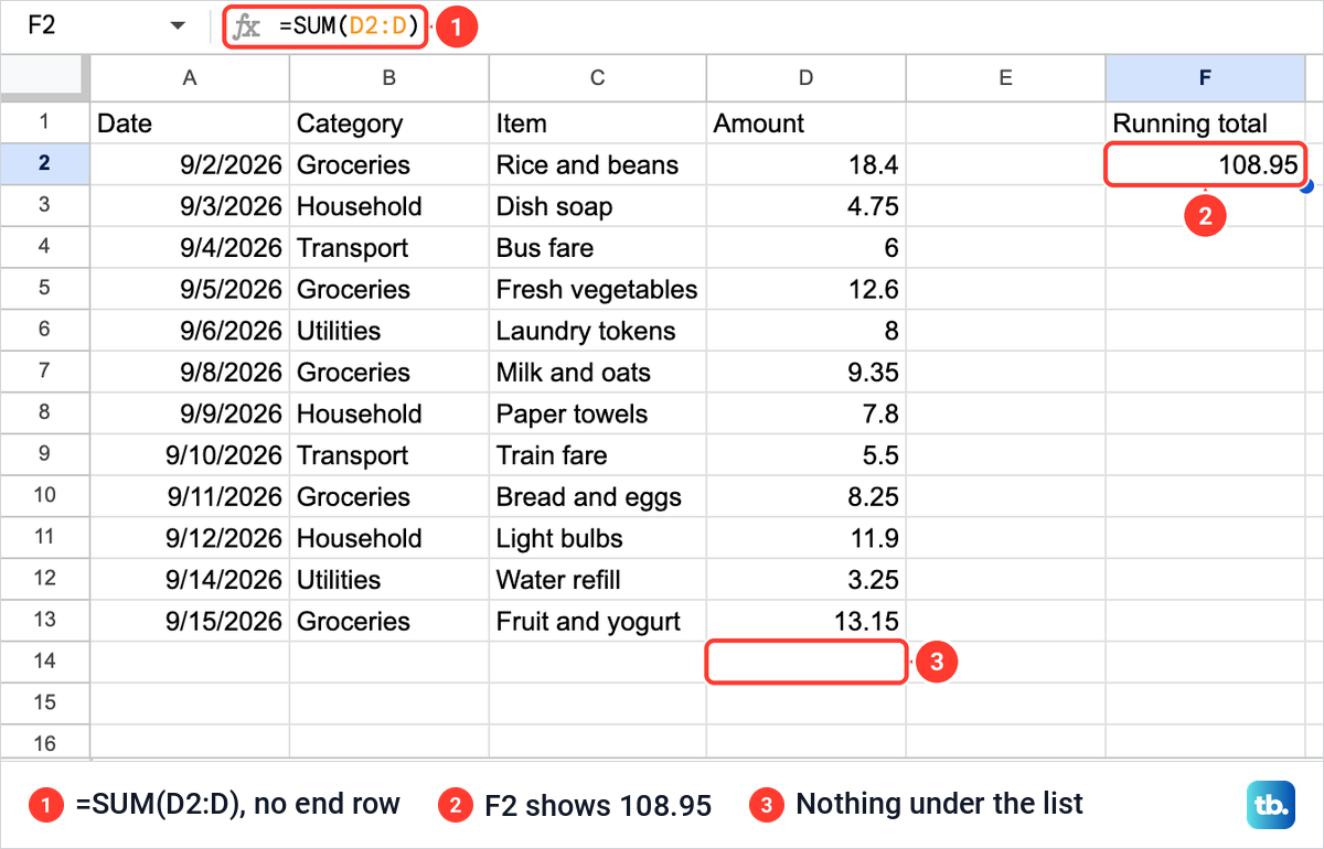
A total under the list has one weakness. The next purchase has nowhere to go but under the total, outside D2:D13. For a list you keep adding to, leave the end row off the range and put the formula in another column. If there is no free column beside the list, add a column in Google Sheets first.
=SUM(D2:D)We cleared D14, typed Running total in F1 and =SUM(D2:D) in F2. It showed 108.95, the same as before, because D2:D means everything from D2 to the bottom of column D.
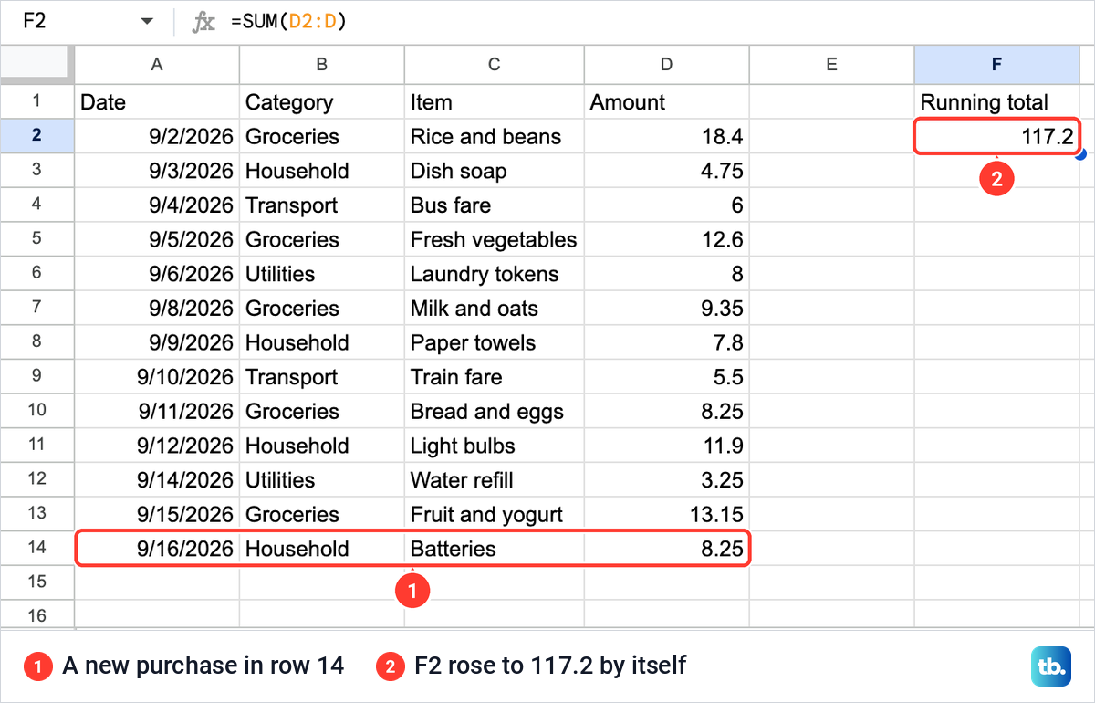
Then we typed a 13th purchase in row 14, Batteries for 8.25. F2 rose to 117.2 by itself, with no change to the formula. We cleared the row again afterwards.
If you would rather keep the total under the list, add rows above it. Make room with our guide to insert multiple rows in Google Sheets, then click the total and check that the range in the formula bar still reaches the last amount. If it stops short, edit the range so it ends at the last amount, the row just above the total.
Why a whole column total shows an error or doubles
An open-ended range must not sit in its own column. When we typed =SUM(D2:D) into D14, the cell showed #REF! with a red corner. Resting the pointer on it showed "Circular dependency detected. To resolve with iterative calculation, see File > Settings."
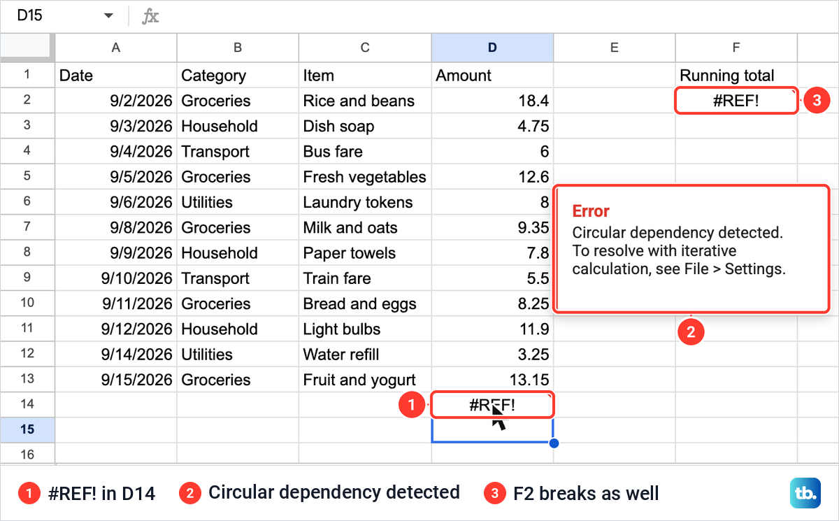
The formula in D14 was trying to add itself. F2, which read column D, turned to #REF! as well, so one wrong cell broke both totals. Skip the iterative calculation hint for a simple total, delete the formula from column D and put it in another column.
The second trap shows no error at all. We put the ordinary total back in D14, =SUM(D2:D13), and kept =SUM(D2:D) in F2. F2 read 217.9, exactly double, because the open-ended range also added the total at the bottom of the amounts.
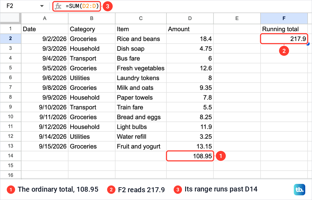
So use one style per column: a fixed total under the list, or an open-ended total somewhere else, never both. The same goes for any other number you type under the amounts, since D2:D adds every number in the column.
Total one category with SUMIF
To add up only some rows, use SUMIF. It takes three parts: the column to check, the word to look for and the column to add.
=SUMIF(B2:B13,"Groceries",D2:D13)In F2 of our sheet this gave 61.75, the five Groceries rows: Rice and beans, Fresh vegetables, Milk and oats, Bread and eggs, and Fruit and yogurt. Type the word between straight double quotes, spelled as it is in the column.
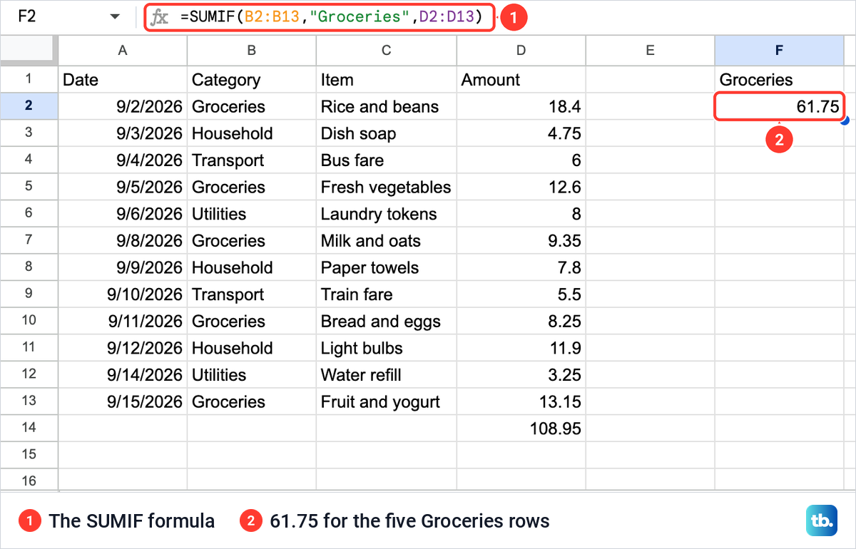
SUMIF only adds rows whose category matches that word, so a row typed as Grocery would be left out. A drop-down list in Google Sheets for the Category column keeps every entry spelled the same way. Once each category has its own total, you can make a graph in Google Sheets to compare them.
Total only the rows a filter shows
A plain SUM keeps adding every row in its range, including rows a filter hides. To total only the rows left on screen after filtering, use SUBTOTAL with the code 9, which stands for sum.
=SUBTOTAL(9,D2:D13)Rows hidden by a filter are never included, whatever code you use. For rows you hid by hand, write 109 instead of 9. SUBTOTAL also skips any cell in its range that holds another SUBTOTAL, so a subtotal is not counted twice.
Fix a total that looks wrong
Start by clicking the total and reading its range in the formula bar. A range that stops one row short leaves the last amount out, and one that reaches into its own cell causes the errors above.
Then look at how the amounts sit in their cells, since by default Sheets puts numbers on the right and text on the left. We retyped 12.6 in D5 with an apostrophe in front, which stores it as text. It moved to the left of the cell, and both totals dropped without any warning: 108.95 became 96.35, and the Groceries total went from 61.75 to 49.15.
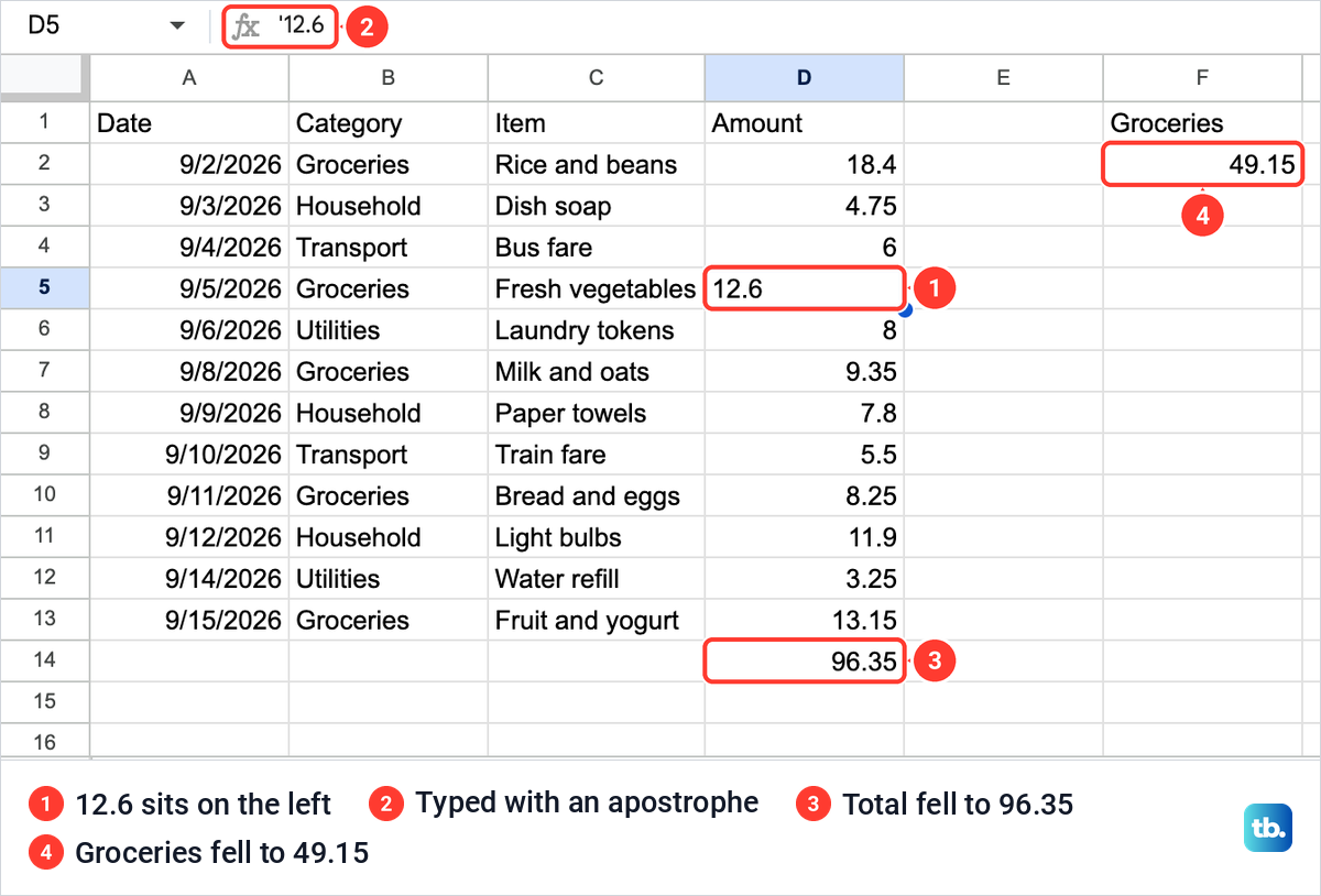
If the amount was typed with an apostrophe, as ours was, the formula bar shows it. Retype the amount as a plain number. We pressed Command + Z to put the number back, which is Ctrl + Z on Windows and ChromeOS.
For a whole column of text amounts, use the VALUE function. In an empty column, =VALUE(D5) turns the text in D5 into a number Sheets can add; fill it down and total that column instead.
Two more causes have nothing to do with formulas. A purchase entered twice is counted twice, so remove duplicates in Google Sheets before you trust the result. To check one group of rows by eye, sort the list in Google Sheets by Category so they sit together. In a long list, freeze a row in Google Sheets so the Category and Amount headings stay in view while you scroll.
Total a column on Android, iPhone and iPad
In the Google Sheets app on an Android phone or tablet, open the spreadsheet and select the cells you want to add up. A row of calculations appears at the bottom, with Sum, Average, Maximum, Minimum and Count. To keep one of them, drag it into a cell, and tap the Formula icon if you want to hide the row.
For a formula, tap the empty cell under the numbers, enter =SUM(D2:D13) with your own range and tap Done. You can also tap Function and pick SUM from a category instead of typing it.
On an iPhone or iPad the steps are the same. Select the cells to see the row of calculations at the bottom, drag a result into a cell to keep it, or tap a cell, type the formula and tap Done.
How we tested this guide
We tested this in Google Sheets on the web in Chrome on a Mac, totaling a column of 12 purchase amounts with SUM, the Sum box, an open-ended range and SUMIF.
Frequently Asked Questions
How do I total an entire column in Google Sheets?
For a list with a fixed end, type =SUM(D2:D13) in the cell under it. For a column you keep adding to, type =SUM(D2:D) in a cell of another column, which picked up a new row by itself in our sheet. Keep the open-ended formula out of the column it adds, and do not keep a second total in that column.
Can I see the sum of a column without a formula?
Yes. Select the numbers and read Sum in the box at the bottom right of the window, and click it for the average, smallest and largest amount and the count. In the phone app, a row of calculations appears at the bottom when you select cells.
Why is my SUM total too low?
An amount may be stored as text. It sits on the left of its cell by default, and in our sheet one such amount pulled the total from 108.95 down to 96.35 with no error. Retype it as a plain number, then check that the range in the formula reaches the last row.
Why does my total say circular dependency detected?
The formula sits inside the range it adds, for example =SUM(D2:D) in column D. Move it to a cell in another column. In our sheet the cell showed #REF!, and the other total that read column D broke with it.
Why is my whole column total double?
The column already holds another total, and the open-ended range adds it too. Ours read 217.9 instead of 108.95. Keep one kind of total: remove the total under the list, or give the other formula a fixed end row such as D13.
How do I total only one category?
Use SUMIF with the category column, the word and the amount column, such as =SUMIF(B2:B13,"Groceries",D2:D13). In our sheet it gave 61.75 for the five Groceries rows.
How do I total only the rows a filter shows?
Use =SUBTOTAL(9,D2:D13) instead of SUM. Rows hidden by a filter are left out, and the code 109 also leaves out rows you hid by hand.