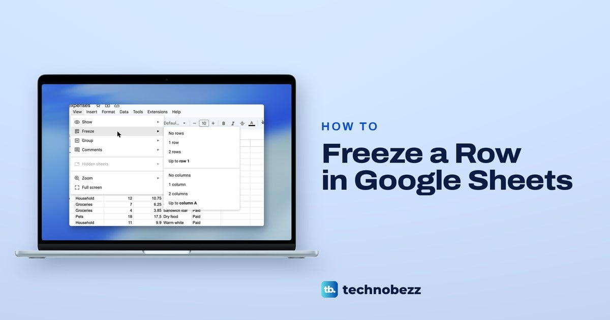
To freeze a row in Google Sheets on a computer, click View > Freeze > 1 row. A thick grey line appears under row 1, and that row stays put as you scroll. To keep more than one row, click a cell in the last row you want to keep and choose the Up to row entry from the same menu.
We froze and unfroze rows in Chrome on our Weekly expenses sheet, a list of 18 household purchases with its headings in row 1. Two things in the menu are easy to miss: the Up to row entry follows whichever cell is selected, and unfreezing the rows leaves a frozen column exactly where it was.
The short version
- Top row: click View > Freeze > 1 row.
- Several rows: click a cell in the last row to keep, then choose View > Freeze > Up to row and its number.
- Unfreeze: choose View > Freeze > No rows. A frozen column stays until you choose No columns.
- Phone or tablet: on Android, touch and hold the row and tap Freeze. On iPhone or iPad, tap the row number, tap the right arrow, then Freeze.
- Printing: Repeat frozen rows in the Sheets print settings puts the frozen row at the top of every page.
Freeze options at a glance
| What you want | Where | What to choose |
|---|---|---|
| Keep the top row in view | Computer | View > Freeze > 1 row |
| Keep a title row and the headings | Computer | View > Freeze > 2 rows |
| Keep every row down to a chosen row | Computer | Click a cell in that row, then View > Freeze > Up to row and its number |
| Keep the first column as well | Computer | View > Freeze > 1 column |
| Stop freezing rows | Computer | View > Freeze > No rows (frozen columns stay) |
| Freeze or unfreeze a row | Android app | Touch and hold the row, then tap Freeze or Unfreeze |
| Freeze or unfreeze a row | iPhone or iPad app | Tap the row number, tap the right arrow, then Freeze or Unfreeze |
| Print the frozen row on every page | Computer | File > Print > Headers & footers > Repeat frozen rows |
Freeze the top row on a computer
Open the spreadsheet in your browser. Click View in the menu bar, point to Freeze, and choose 1 row from the list that opens beside it.
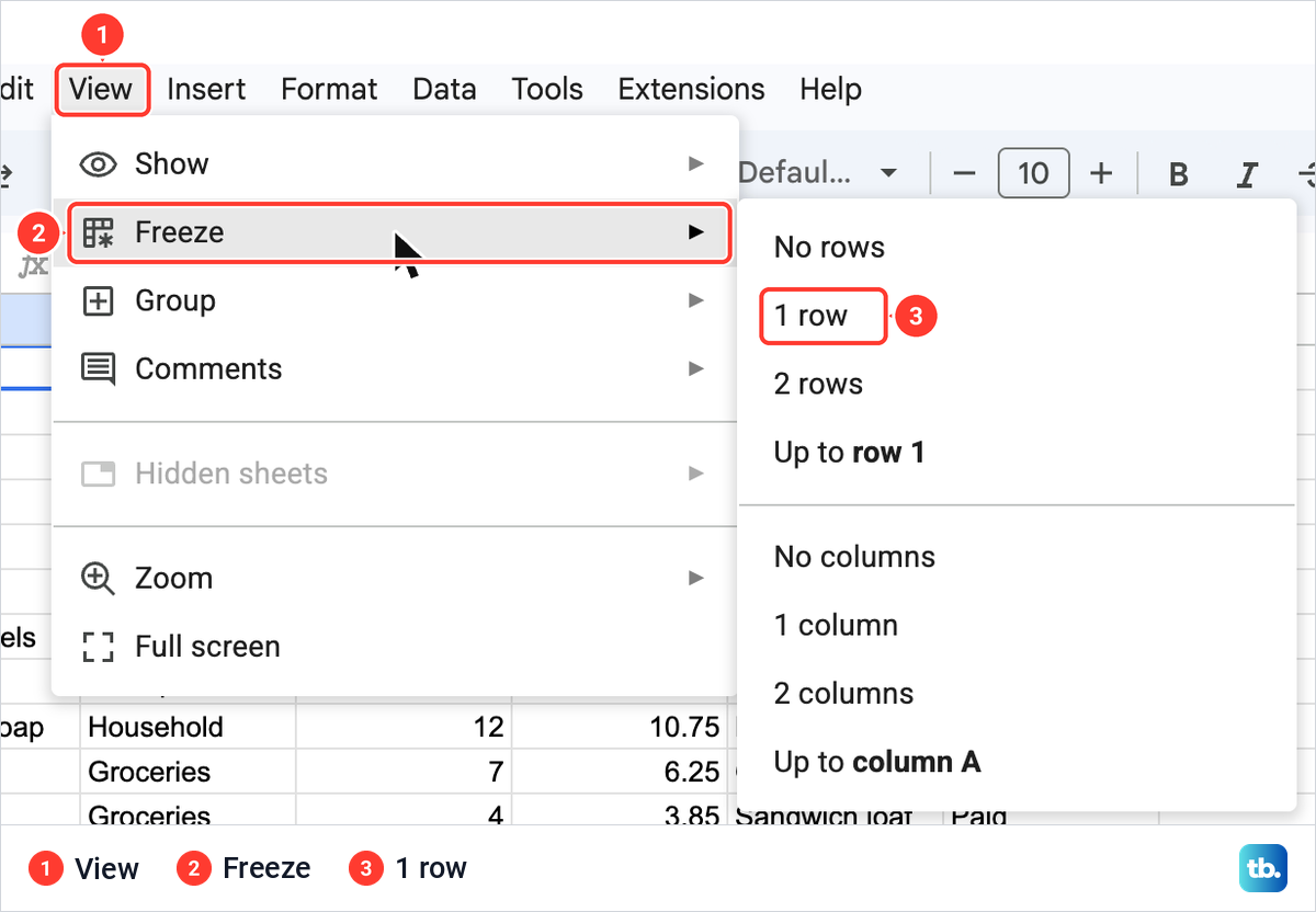
The Freeze list has two groups of four. The rows group reads No rows, 1 row, 2 rows and an Up to row entry, and the columns group below it repeats the same pattern for columns. Nothing changes in the sheet until you click one of them.
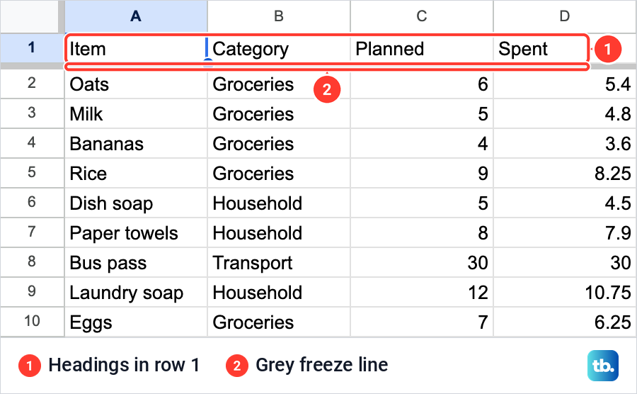
As soon as we chose 1 row, a thick grey line appeared under row 1. Everything above that line is frozen. When you open a sheet someone else set up, that line is the quickest way to see what they froze.
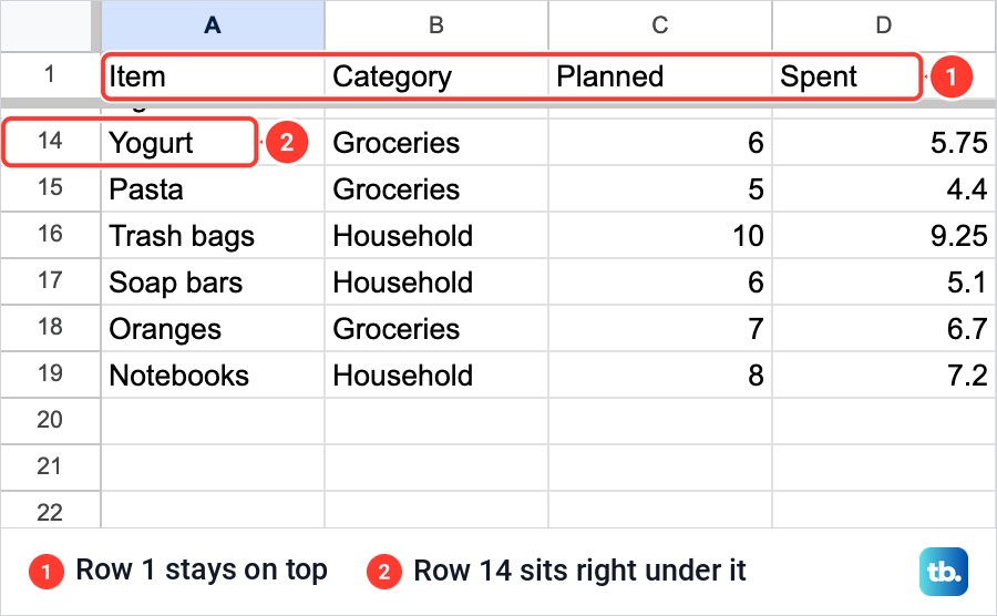
Now scroll down to check it. We jumped down to cell A30, and row 1 with the headings Item, Category, Planned and Spent stayed in place under the column letters. Row 14 sat right under the line, so every amount still had its heading above it.
A frozen heading row also helps when you alphabetize and sort in Google Sheets. If your sheet has headings, freeze the first row, and when you sort a range with Data > Sort range, tick Data has header row as well.
Freeze two or more rows
If your sheet has a title in row 1 and the headings in row 2, choose 2 rows from the same list. For anything deeper, use the fourth entry in the rows group. Its label is not fixed, and that is what makes it useful.
With cell A1 selected, our menu read Up to row 1. When we clicked cell B3 and opened View > Freeze again, the same entry read Up to row 3, and the columns entry read Up to column B. So click any cell in the last row you want to keep, then choose Up to row and its number.
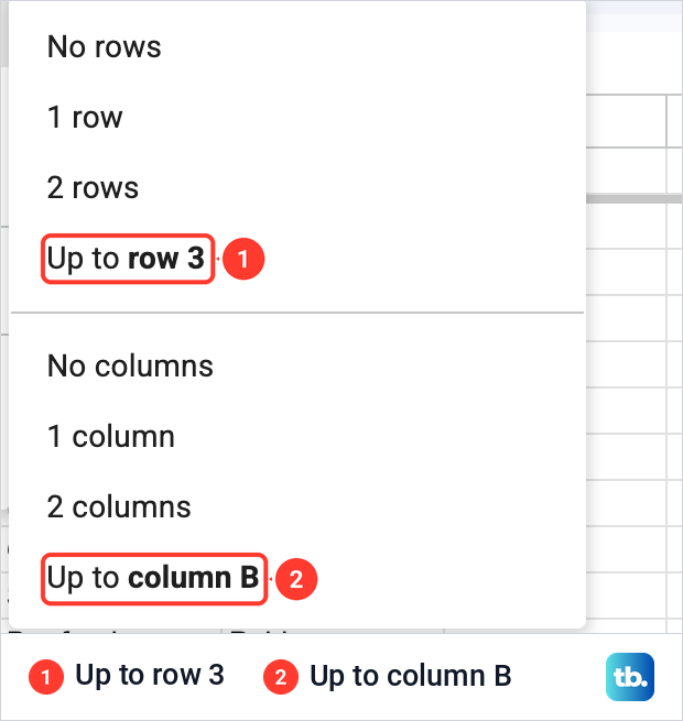
We chose Up to row 3 and the grey line moved from under row 1 to under row 3, with no need to unfreeze first. Rows 1, 2 and 3 all stayed put. The menu only counts rows from the top, so freezing up to row 5 keeps rows 1 to 5, and there is no way to hold row 5 on its own.
Freeze a column at the same time
Rows and columns are frozen separately, so a sheet can have both. With rows 1 to 3 already frozen, we chose View > Freeze > 1 column. A second grey line appeared to the right of column A, and the line under row 3 stayed where it was.
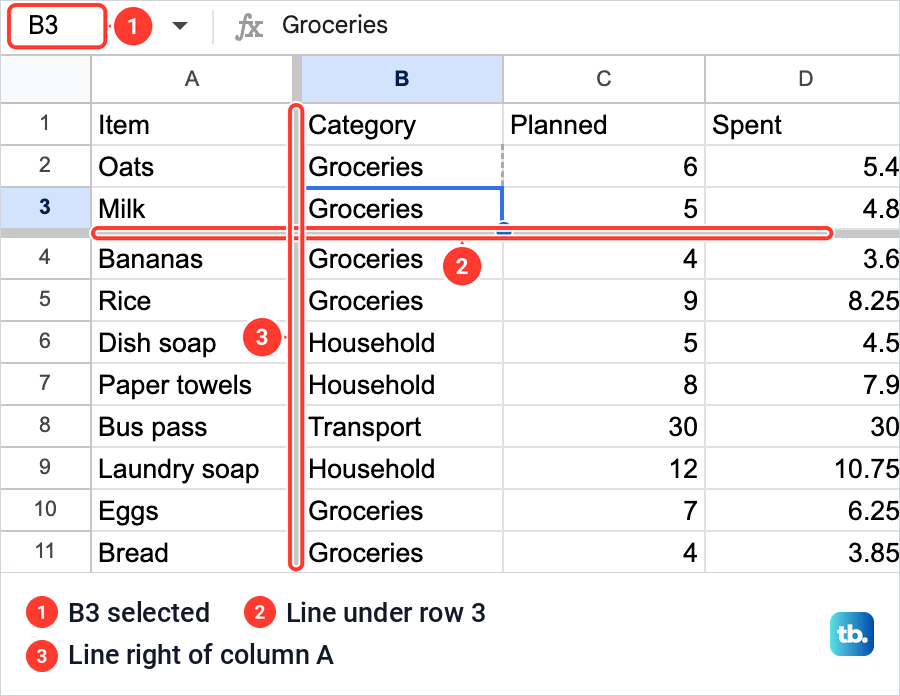
This suits a wide sheet whose first column holds the names of things. Frozen rows and columns stay on screen as you scroll, so the item names stay in view as you move right and the headings stay as you move down. The columns group also has a 2 columns entry and its own Up to column entry.
Unfreeze rows in Google Sheets
To unfreeze, open View > Freeze and choose No rows. The columns group has its own No columns entry, and you need it if a column is frozen too.
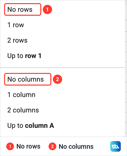
The two really are separate. When we chose No rows on our sheet with three rows and one column frozen, the line under the rows disappeared but column A stayed frozen. Only No columns cleared that second line.
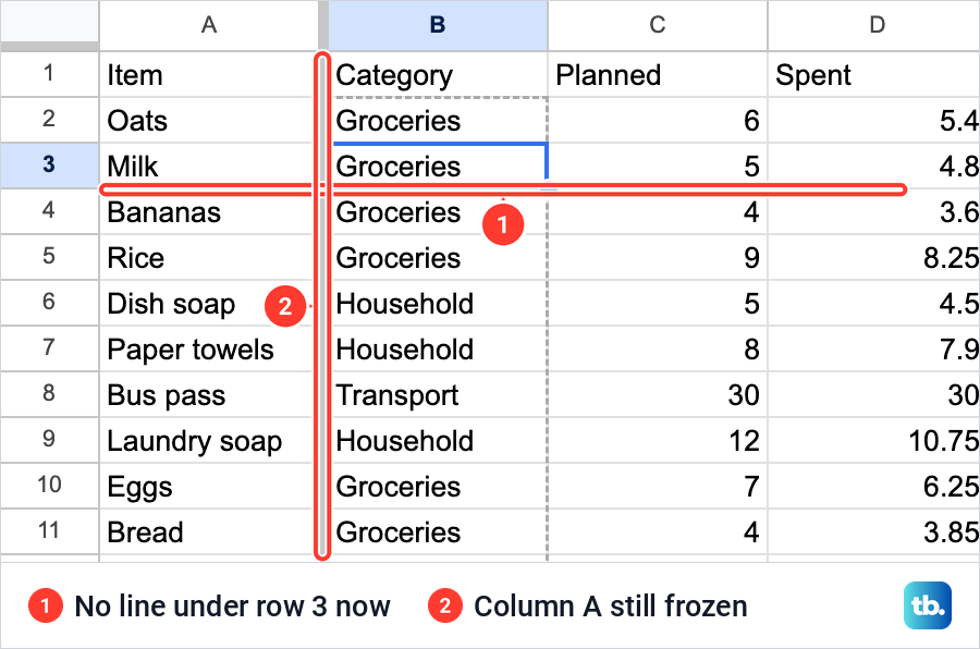
You do not have to unfreeze before changing the count. Pick 1 row or 2 rows, or click a cell in the new last row and choose its Up to row entry, and the grey line moves to match.
Freeze a row in the Google Sheets app
The Sheets apps for Android and iPhone use different steps. On an Android phone or tablet, open the spreadsheet in the Google Sheets app, touch and hold a row, and tap Freeze in the menu that appears. To undo it, touch and hold the row again and tap Unfreeze.
On an iPhone or iPad, open the spreadsheet in the Sheets app and tap a row number. In the menu that appears, tap the right arrow, then tap Freeze or Unfreeze.
If Freeze is missing from that menu on your iPhone, one more thing to try is to update an app on iPhone and look again. If the menu does not appear when you touch and hold a row on Android, clear an Android app cache and reopen the spreadsheet.
Repeat the frozen row on printed pages
Freezing is about the screen, but Sheets also uses it when you print. To print the frozen row on every page, click File > Print, open Headers & footers and tick Repeat frozen rows. On our Mac, pressing Cmd + P opened the same Print settings view inside Sheets.
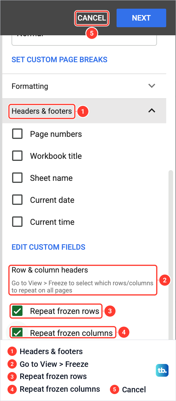
Under Row & column headers, the panel says Go to View > Freeze to select which rows/columns to repeat on all pages. Repeat frozen rows and Repeat frozen columns were both already ticked when we opened it. Before you print, check that Repeat frozen rows is ticked on your own sheet. When we were done, Cancel closed Print settings.
If you want the headings on the first page only, untick Repeat frozen rows. If the printer then shows as unavailable when you continue, here is how to fix a printer that shows offline.
When the wrong rows stay in place
If more rows are frozen than you wanted, the Up to row entry is a likely cause, because it follows whichever cell was selected when you clicked it. Find the grey line first, then open View > Freeze and choose 1 row, 2 rows or No rows to reset it.
Freezing does not stop anyone from changing those rows. It only decides what stays on screen. To limit who can edit the headings, use Data > Protect sheets and ranges, which opens a panel on the right where you pick the range and set its permissions.
Freezing is not hiding either. A hidden row drops out of view until you show it again, while a frozen row is always on screen. To hide a row instead, right-click it and choose Hide row.
To show a colleague where the grey line sits, take a screenshot on a Mac or take a screenshot on Windows. With the headings fixed in place, the same table is ready when you want to make a graph in Google Sheets.
How we tested this guide
We tested this in Google Sheets on the web in Chrome on a Mac, freezing and unfreezing rows and a column in a 19-row expenses sheet.
Frequently Asked Questions
How do I freeze the top row in Google Sheets?
On a computer, click View, point to Freeze and choose 1 row. A thick grey line appears under row 1, and that row stays at the top while you scroll.
How do I freeze more than one row?
Choose 2 rows from View > Freeze, or click a cell in the last row you want to keep and choose the Up to row entry. That entry names the row of the selected cell, so with B3 selected it reads Up to row 3.
Can I freeze a row in the middle of a sheet on its own?
No. Freezing always counts from row 1, so freezing up to row 5 keeps rows 1 to 5 in view. If the rows above it get in the way, move the row you need to the top first.
How do I unfreeze rows in Google Sheets?
On a computer, click View > Freeze > No rows. A frozen column is cleared separately with No columns. In the Android app, touch and hold the row and tap Unfreeze, and on an iPhone or iPad, tap the row number, the right arrow, then Unfreeze.
Does freezing a row stop other people from editing it?
No. Freezing only keeps rows on screen while you scroll. To control who can change them, use Data > Protect sheets and ranges.
Why does my frozen header row print on every page?
That happens when Repeat frozen rows is ticked in the Sheets print settings, and it was already ticked when we opened them on our sheet. Open File > Print, expand Headers & footers and untick Repeat frozen rows to stop it.