
To alphabetize in Google Sheets, select the whole table with its headings, open Data > Sort range > Advanced range sorting options, tick Data has header row, choose the column to sort by and A to Z, then select Sort. Every row moves as one, so each item keeps its own numbers and notes. Tick the header setting yourself, because it was off when we opened the sort options, even though our heading row was frozen.
Sheets can also sort by two columns at once, sort a whole tab from a column letter, or build a sorted copy with the SORT function while the original stays as it is. We sorted our Weekly expenses sheet by one column, by two columns and with SORT. The one mistake to know before you start is selecting a single column of a table, because Sheets sorted it on its own, without a warning, and every row came apart.
The short version
- Select the whole table, then choose Data > Sort range > Advanced range sorting options.
- Tick Data has header row if row 1 holds headings. It was off when the box opened, even with row 1 frozen.
- Never select just one column of a table. Sheets sorts that column alone and the rows no longer match.
- Use Add another sort column to sort by category, then by name inside each category.
- Type =SORT(A2:F19,1,TRUE) in an empty cell, with your own range, for a sorted copy that leaves the original alone.
- Press Ctrl + Z, or Cmd + Z on a Mac, straight away to undo a sort.
Ways to sort in Google Sheets at a glance
| Method | Where to find it | What changes | Best for |
|---|---|---|---|
| Advanced range sort | Data > Sort range > Advanced range sorting options | The selected rows move, the heading row stays when its box is ticked | Alphabetizing a table safely |
| Two sort columns | Add another sort column, in the same box | Rows are grouped by the first column and ordered by the second inside each group | Category first, then name |
| Sort sheet A to Z | Right-click a column letter | The whole tab is sorted, so freeze the heading row first | A tab that holds one table |
| SORT function | =SORT(A2:F19,1,TRUE) in an empty cell | Nothing moves, a sorted copy appears beside the table | Keeping the original order |
| Filter view | Data > Create filter view, on a computer | Only your own view of the file | Shared spreadsheets |
| Phone app | Tap the column letter twice, then More | The data is sorted by that column | A quick sort on the go |
| Ctrl + Z, or Cmd + Z on a Mac | The keyboard, right after a sort | The last sort is reversed | Fixing a mistake at once |
The ranges in the table match the sheet we used, A1:F19 with headings in row 1. Change them to fit your own data.
Alphabetize a table without mixing up rows
Our Weekly expenses sheet holds a heading row and 18 rows of Item, Category, Planned, Spent, Notes and Status, in A1:F19. The goal was A to Z order by item, with each item keeping its own category, amounts and note.
Select the whole table first. Drag from the first heading to the bottom-right cell, or type the range, such as A1:F19, into the box at the left of the formula bar and press Enter. Every column that belongs to a row must sit inside the selection, or it stays behind while the rest moves.
With the table selected, open the Data menu, point to Sort range and select Advanced range sorting options. The two entries above it, Sort range by column A (A to Z) and (Z to A), sort at once by the column their names show, with no header box to tick.
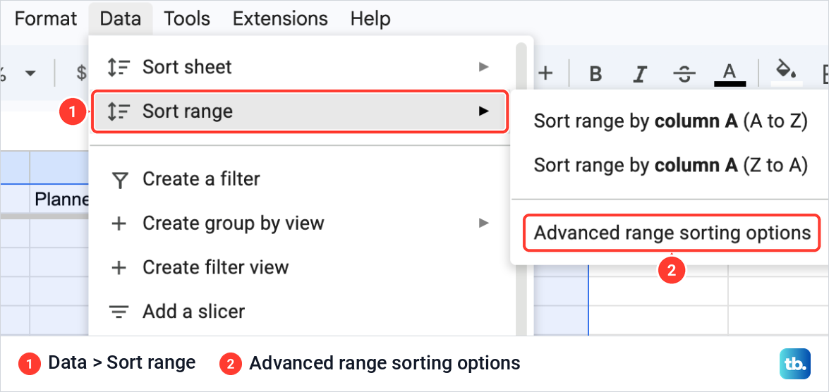
Tick Data has header row yourself
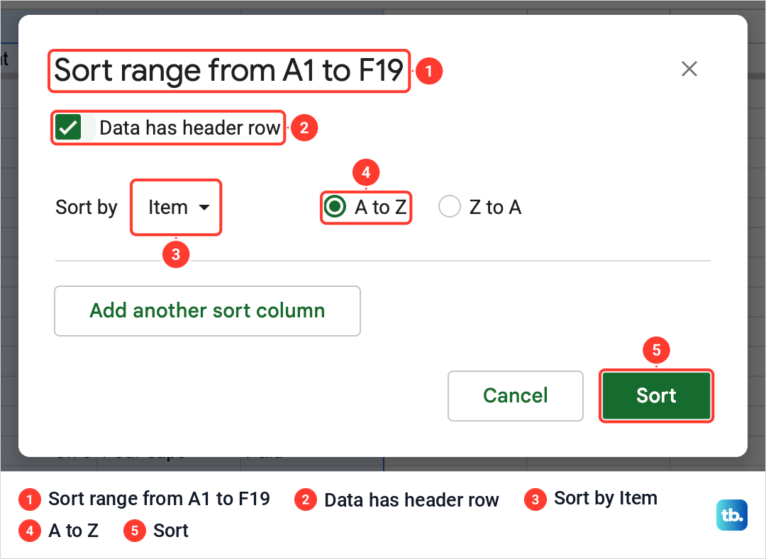
The box that opens names the range, and ours read Sort range from A1 to F19. Below the title is Data has header row, which was not ticked when the box opened, although row 1 of our sheet was frozen. Until we ticked it, the Sort by list offered Column A rather than Item, so the headings would have been sorted in with the data.
Tick it if row 1 holds headings, and leave it clear if your first row is data. The list then shows your heading names. Choose the column to sort by, here Item, choose A to Z, or Z to A for reverse order, and select Sort.
Freezing the first row of a sheet with headings keeps them in view as you scroll, and it is worth doing as well. On our sheet the frozen row did not tick the header box, so treat the two as separate steps.
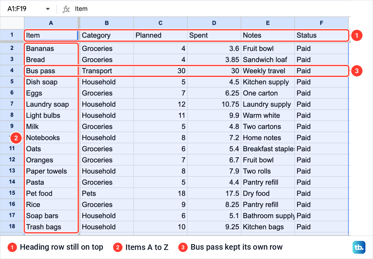
After the sort, the heading row stayed on top and the items ran from Bananas, Bread and Bus pass down to Trash bags and Yogurt. Each row came along whole, and Bus pass still sat beside Transport, 30, 30 and Weekly travel. Check one familiar row like that after any sort, because it is the quickest way to spot a selection that missed a column.
Sort by two columns
A second sort column decides the order inside groups. Open Advanced range sorting options on the whole table again, tick Data has header row, set Sort by to Category and A to Z, then select Add another sort column. Set the new then by row to Item and A to Z, and select Sort.
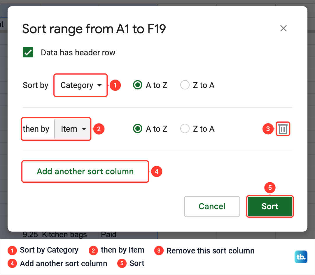
A bin button at the end of the second row removes it again, and Add another sort column stays available for a third key. Our result put the Groceries rows first, Bananas to Yogurt in item order, then Household from Dish soap to Trash bags, then Pets and Transport.
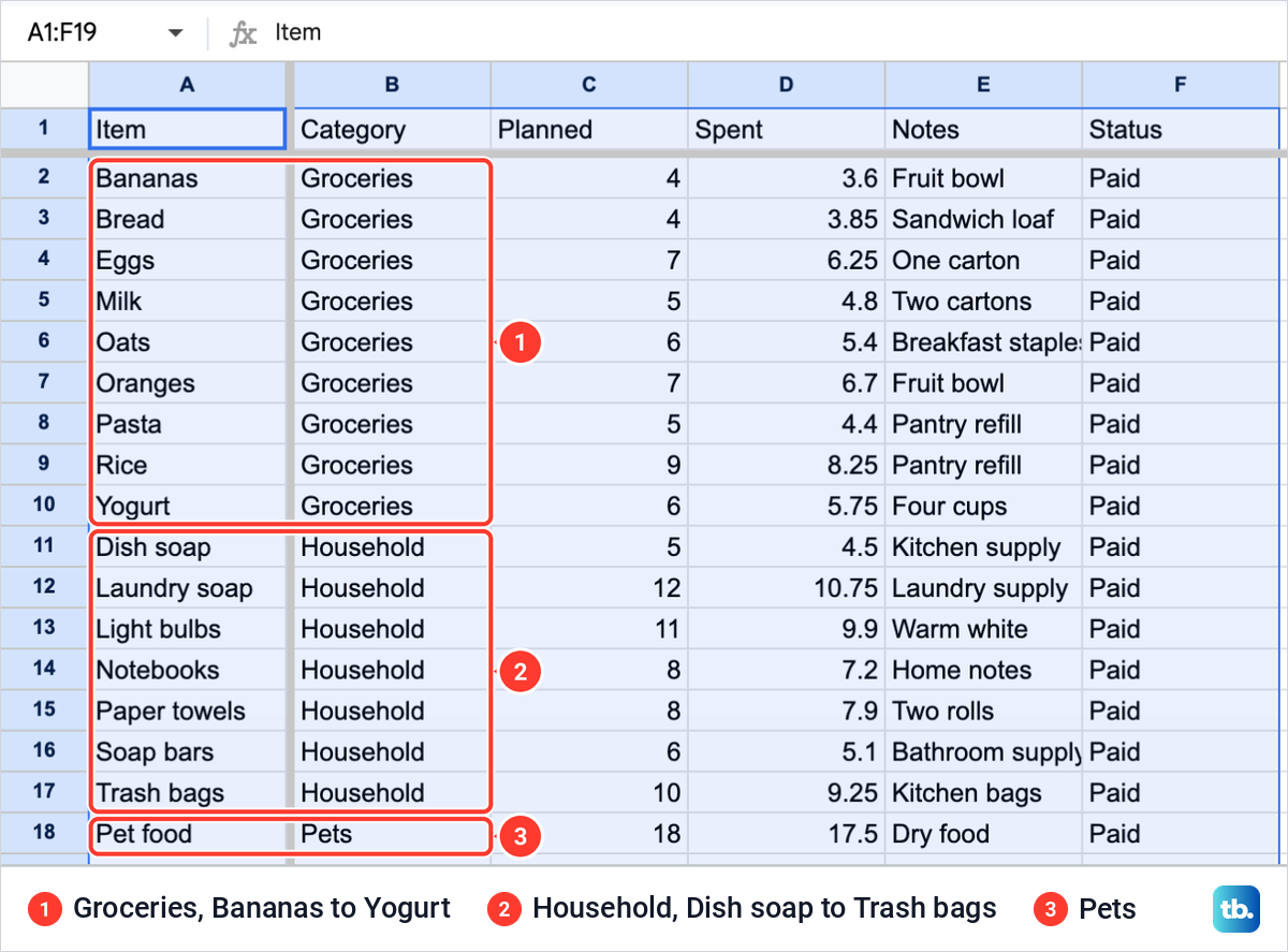
Groups only form when entries are spelled the same way, so Grocery and Groceries would land in different places. Fix the spelling first, then sort. With the categories grouped, you can make a graph in Google Sheets that compares them.
Sort the whole sheet from a column letter
For a tab that holds one table and nothing else, there is a shortcut. Right-click the letter at the top of the column to sort by, such as A, and choose Sort sheet A to Z or Sort sheet Z to A. On our sheet both entries sat in the column menu between Create a filter and Conditional formatting.
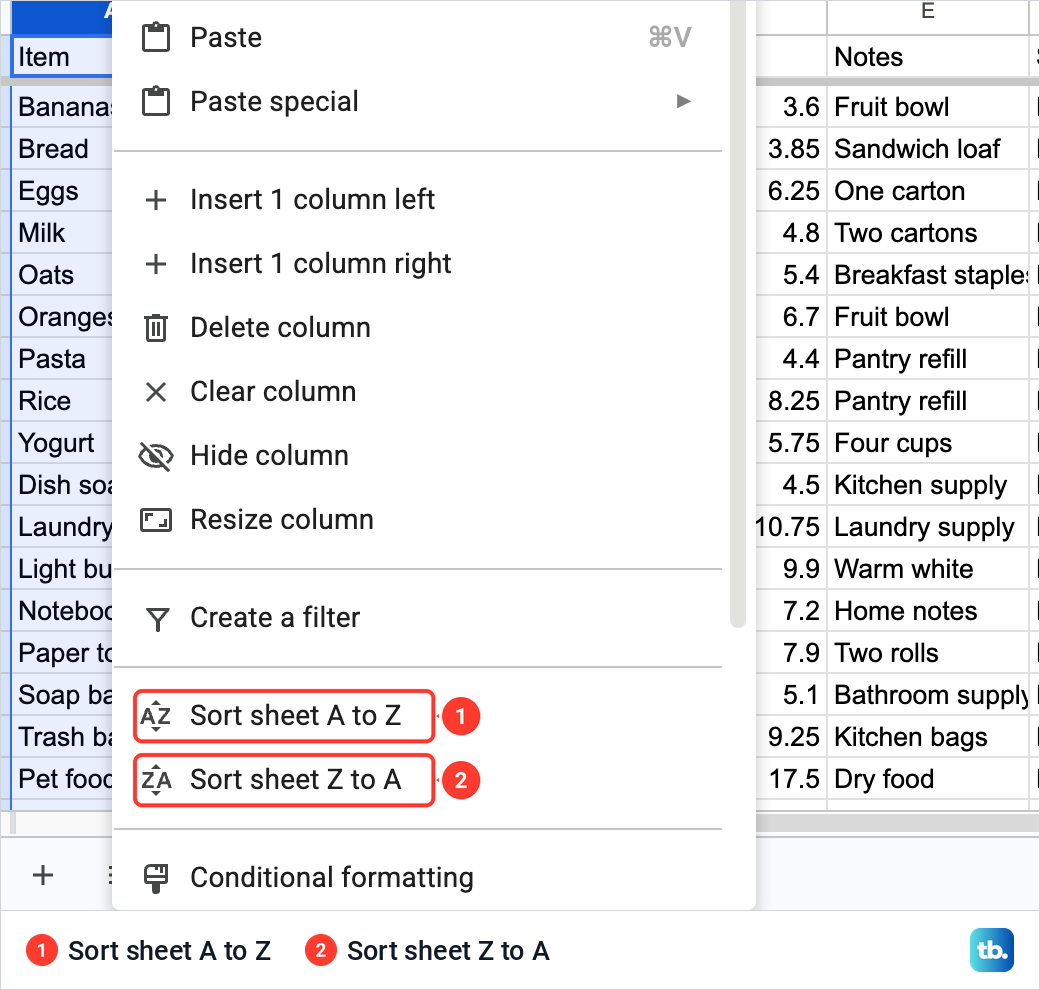
Sort sheet works on the whole tab rather than a selection, so any other list on the same tab is reordered with it. On a sheet with a header row, freeze the first row before sorting, with View > Freeze > 1 row, so the heading row stays at the top instead of being sorted in with the data. The Data menu has a Sort sheet entry as well, just above Sort range.
Why sorting one column scrambles your rows
This is the easiest way to wreck a list. We selected only the item names, A2:A19, and chose Data > Sort range > Sort range by column A (Z to A). Sheets reordered those 18 cells, left columns B to F exactly where they were and showed no warning first.
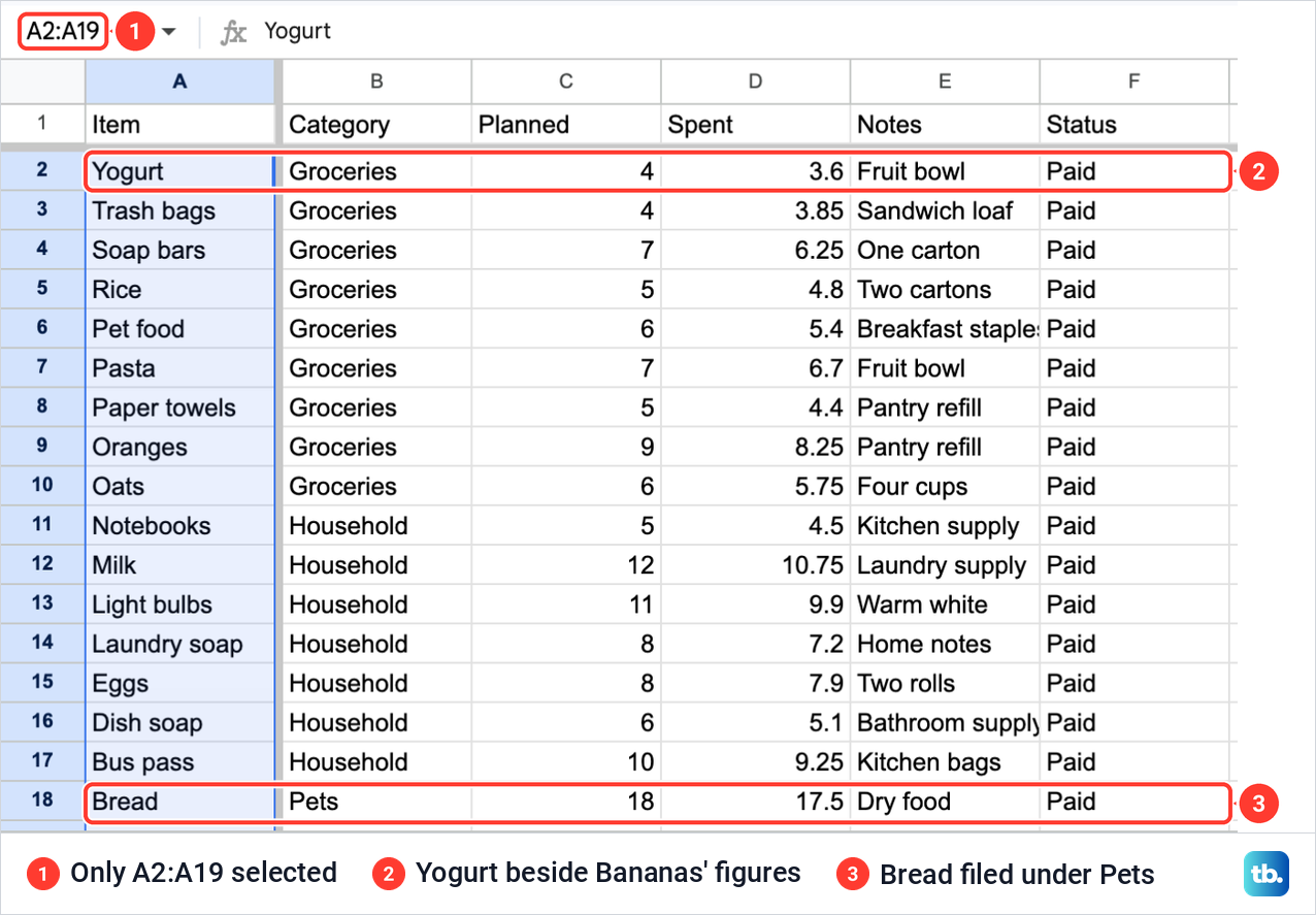
Every row was now wrong. Yogurt sat beside the 4, 3.6 and Fruit bowl that belonged to Bananas, Trash bags was filed under Groceries, and Bread ended up in the Pets row with the dry food. Nothing on screen flags the damage, so a look at one familiar row is the only check.
Press Cmd + Z on a Mac, or Ctrl + Z on Windows and ChromeOS, straight away. On our Mac, Cmd + Z put every item back beside its own figures in one step. Then select the whole table and sort again from Advanced range sorting options.
Keep the original order with the SORT function
The SORT function builds a sorted copy and leaves the table alone, which suits a shared sheet or a list whose entry order matters. Click an empty cell with free space below it and to its right, and type the formula with your own range, leaving out the heading row.
=SORT(A2:F19,1,TRUE)We typed it in H2. Sheets filled H2:M19 with all 18 rows in item order, Bananas, Bread, Bus pass and on down, while the table in columns A to F kept its own order. The copy has no headings, so type them into row 1 above it.
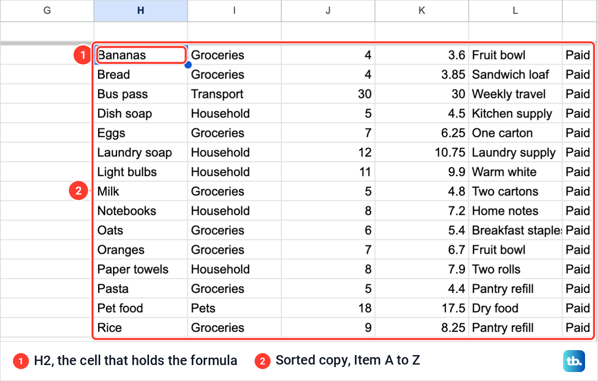
The 1 is the column to sort by, counted from the left edge of the range, and TRUE means A to Z, while FALSE means Z to A. The function takes more pairs for tie-breakers, so =SORT(A2:F19,2,TRUE,1,TRUE) would sort by Category and then by Item. Only the columns named in the formula decide the order, and the other fields stay with their rows, as Bus pass kept Transport, 30, 30 and Weekly travel in our copy.
Because the copy is a formula, it depends on the source rows. Keep the original table in place while you use the result, and edit the source rather than the copy.
Sort without changing what others see
In a shared file, a sort in the table changes the order for everyone who opens it. The way round that is a filter view. On a computer, choose Data > Create filter view, sort inside the view, then select Save View at the top right and Save. A filter view applies only to your view of the spreadsheet, and the entry sits in the same Data menu as Sort range.
A plain filter works differently. Anyone with access to the spreadsheet sees a filter you add, and anyone who can edit the file can change it. If you can only view a file, you can still create a temporary filter view that only you can use, though it is not saved.
Sort in the Google Sheets app on Android and iPhone
The phone apps sort from the column menu. Filter views are not part of the apps and need Sheets on a computer.
Android phone or tablet
Open the spreadsheet in the Sheets app and tap the letter at the top of the column to select it. Tap the top of the column again to open its menu, then tap More. Scroll down and tap SORT A-Z or SORT Z-A.
iPhone and iPad
On iPhone and iPad the steps are almost the same. Tap the column letter, tap the top of the column again, tap More, the right-arrow at the end of the menu, and then SORT A-Z or SORT Z-A. There is no scroll step in between.
The apps do this one-column sort only. The header setting and extra sort columns of Advanced range sorting options are on the computer, so for a table with headings or a two-column sort, open the file in Sheets on a computer. Check one familiar row after a phone sort, just as on the web.
Undo a sort or get the old order back
Undo is the fastest fix. Press Ctrl + Z on Windows and ChromeOS or Cmd + Z on a Mac right after the sort, which reversed our scrambled one-column sort in one step. A sort is not a setting you can switch off later, because the cells themselves have moved.
If you notice the problem after more edits, check version history for a version with the old order. Open File > Version history > See version history and look through the earlier versions in the right panel. If you find one, make a copy of it to keep your later edits, or select Restore this version. You need permission to edit the file to see its version history.
For a list whose original order matters, such as entries in the order they happened, add a column of row numbers before the first sort. Sorting that column from smallest to largest later puts the rows back the way they came in.
When the order still looks wrong
A stray space is worth checking first when one entry sits out of place. Sheets keeps a space typed in front of a word, and on another of our sheets a leading space stayed in the cell until Data > Data cleanup > Trim whitespace removed it. Run Trim whitespace on the column, then sort again.
Formulas can catch you out too. When a formula points to a cell inside a filtered range, sorting that range does not change the formula, so =B2 still reads =B2 and shows whatever value moved into B2. Check formulas like that after a sort.
Names are another case. A cell that holds a first and last name sorts by the first name, so to alphabetize by surname, insert an empty column to the right of the names, so the split does not write over the next column. Then select the names and choose Data > Split text to columns. Use the menu next to Separator to make Sheets split at the space, then check any name with a middle name or a two-word surname before you sort.
If the list is still in Excel, you can split the cells into separate Excel columns there, and combine two columns in Excel later if you want full names back in one cell. Either way, sort by the surname column with the whole table selected.
Prepare a list from Excel or a PDF
A plain table is the easiest to sort: one heading row, one record per row and no empty rows in the middle, so a single drag selects all of it. If your list only exists as a table in a PDF, convert the PDF to Excel first, then bring the workbook in with File > Import.
Check the workbook in Excel before it comes across. Unhide the hidden columns in Excel so every field is in view when you select the table. If a title is merged across the top, check how you merge cells in Excel without losing data, and keep that title row outside the range you sort.
Sorting also brings repeated entries together, which makes them easy to spot. Data > Data cleanup > Remove duplicates removes rows with repeat data, so select the whole table and set the header option and the columns to compare before you confirm. For a list that still lives in Excel, you can remove duplicates in Excel before the import.
How we tested this guide
We tested this in Google Sheets on the web in Chrome on a Mac, sorting an 18-row expenses sheet by one column, by two columns and with the SORT function.
Frequently Asked Questions
How do I alphabetize in Google Sheets without mixing up rows?
Select every column of the table, not only the one you want in order, then use Data > Sort range > Advanced range sorting options. When we sorted one column on its own, Sheets moved only that column and every row came apart.
How do I keep the header row at the top when sorting?
In Advanced range sorting options, tick Data has header row when row 1 holds headings, and leave it clear when it does not. Freezing row 1 is a good habit too, but on our sheet a frozen row did not tick the box for us.
Can I sort by two columns in Google Sheets?
Yes. In Advanced range sorting options, set the first column, select Add another sort column and set the second. Rows that share a value in the first column are then ordered by the second.
How do I sort in Google Sheets without changing the original data?
Type =SORT(A2:F19,1,TRUE) in an empty cell, using your own range, and Sheets builds a sorted copy while the table keeps its order. On a computer, a filter view also lets you sort your own view of a shared file.
How do I alphabetize in the Google Sheets app?
Tap the column letter, tap the top of the column again, tap More and choose SORT A-Z or SORT Z-A. On Android, scroll down before the two sort entries appear.
How do I undo a sort in Google Sheets?
Press Ctrl + Z, or Cmd + Z on a Mac, straight after the sort, which reversed our scrambled sort in one step. Later on, open File > Version history > See version history and look for an earlier version with the old order, then copy or restore it.