To remove duplicates in Google Sheets, select the whole table, open Data > Data cleanup > Remove duplicates, tick Data has header row if your first row holds column names, choose the columns that decide a match and select Remove duplicates. Sheets deletes the repeated rows, keeps the first row of each set and tells you how many it removed. Tick the header box yourself, because it was off by default when we opened the tool.
The same menu can also trim stray spaces, and a formula called UNIQUE builds a clean copy without touching the original. We ran Remove duplicates and UNIQUE on a 16-row pantry list, then added a row with a stray space to try Trim whitespace. Three results are worth knowing before you click: a one-column cleanup deletes whole rows, a leading space hides a duplicate, and Undo brings everything back.
The short version
- Select the whole table, then choose Data > Data cleanup > Remove duplicates.
- Tick Data has header row only if your first row holds column names, otherwise leave it unticked. It is off by default, so headings would be compared as data.
- Leave every column ticked to remove only rows that match in full. With the whole table selected, ticking one column still deletes whole rows that share that value.
- Sheets keeps the first row of each set. Press Ctrl + Z, or Cmd + Z on a Mac, straight away to undo a cleanup.
- To keep the original rows, type =UNIQUE(A1:E17) in an empty cell, using your own table's range.
- On Android, iPhone and iPad, open the spreadsheet in a browser on a computer to remove duplicates.
Ways to remove duplicates in Google Sheets at a glance
| Method | What it does | Your original rows | Best for |
|---|---|---|---|
| Data > Data cleanup > Remove duplicates | Deletes rows that match in the columns you tick, keeping the first of each set | Changed, repeats are deleted | Cleaning the list itself |
| =UNIQUE(A1:E17) in an empty cell | Lists each distinct row once, somewhere else | Untouched | Keeping the original as it is |
| Format > Conditional formatting with COUNTIF | Colours values that appear more than once | Untouched | Checking before you delete |
| =UNIQUE(A2:A17,FALSE,TRUE) | Lists only the values that appear exactly once | Untouched | Finding one-off entries |
| Data > Data cleanup > Trim whitespace | Removes leading, trailing and extra spaces | Changed, spaces are removed | Duplicates that refuse to go |
| Ctrl + Z, or Cmd + Z on a Mac | Undoes the last cleanup | Restored | Right after a mistake |
The ranges in the table match the list we used, A1:E17 with column names in row 1. Change them to fit your own sheet.
Remove duplicate rows with Data cleanup
Our list lives in a file called Kitchen Pantry, on a tab named Pantry Items: a header row and 16 rows of Item, Category, Quantity, Unit and Stored in. Rice, Oats and Beans each appear twice with every field identical. Pasta appears three times, twice as 3 boxes and once as 2 boxes, which is the case that catches people out.
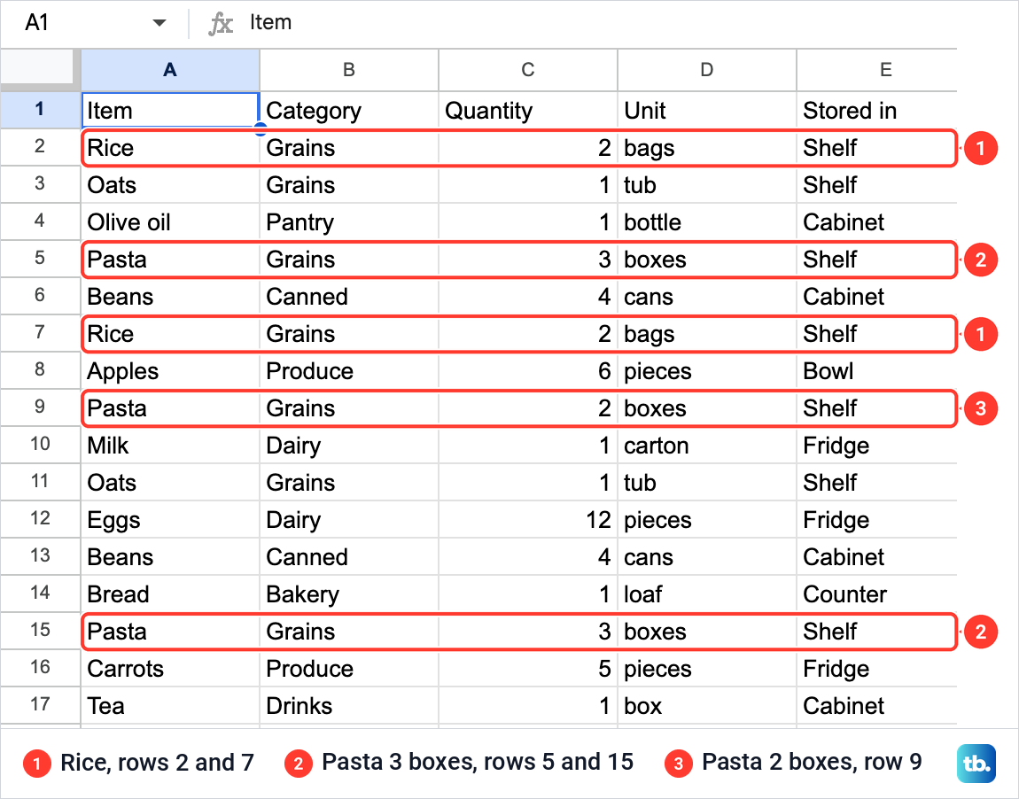
Start by selecting the whole table, headers included. Drag from the first heading to the bottom-right cell so that every column of every row sits inside the blue outline. If you select a single cell inside a range, Sheets removes duplicates for the whole range, but selecting it yourself lets you see exactly what will be compared.
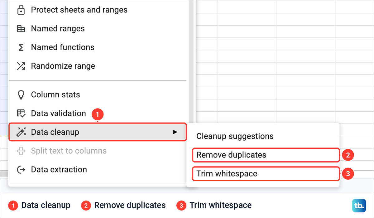
With the table selected, open the Data menu and point to Data cleanup. Three entries appear: Cleanup suggestions, Remove duplicates and Trim whitespace. Select Remove duplicates.
Tick the header box and choose the columns
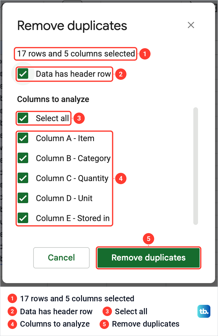
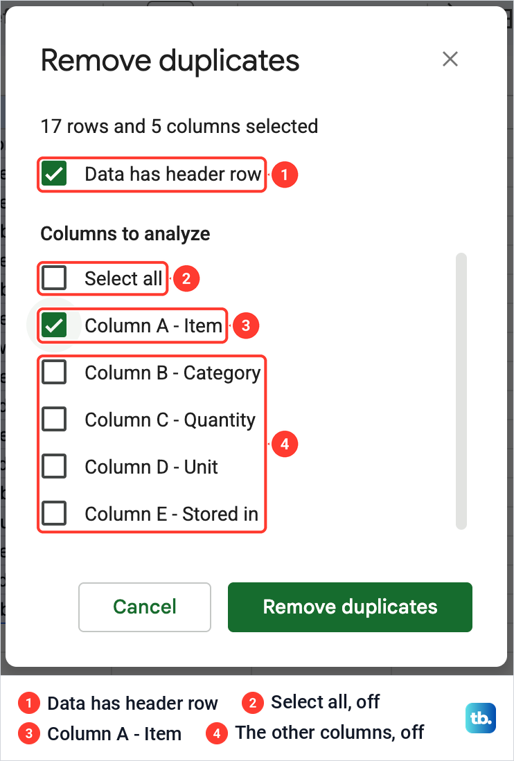
The Remove duplicates box first confirms the selection, and ours read 17 rows and 5 columns selected. Below it is Data has header row, which was not ticked when the box opened. Until we ticked it, the column list read Column A to Column E with no names, and row 1 would have been compared like any other row.
If your first row holds column names, tick it and the list picks up your headings, such as Column A - Item and Column B - Category. Select all and every column are ticked by default, so a row only counts as a duplicate when it matches another row in every column. Leave them that way for a first pass and select Remove duplicates.
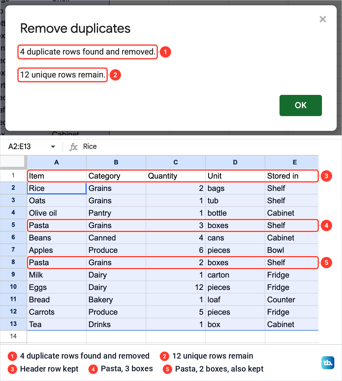
Sheets reported 4 duplicate rows found and removed, 12 unique rows remain. The header stayed in row 1, and the first row of each identical pair stayed: Rice in row 2, Oats in row 3, Pasta at 3 boxes in row 5 and Beans in row 6. The remaining rows moved up to close the gaps, in their original order.
The Pasta row with 2 boxes survived, because its quantity differs and Quantity was one of the ticked columns. That is the safe way to run the tool. Select OK to close the message.
Remove duplicates based on one column
Sometimes you want one row per name, whatever the other fields say. Open Remove duplicates as before, keep Data has header row ticked, untick Select all and tick only the column that should hold each value once, here Column A - Item.
This is where the tool surprises people. On our pantry list it reported 5 duplicate rows found and removed, 11 unique rows remain, and only the first Pasta row, at 3 boxes, was left. The Pasta row with 2 boxes was deleted as a whole row, quantity and all, even though only the Item column was being compared.
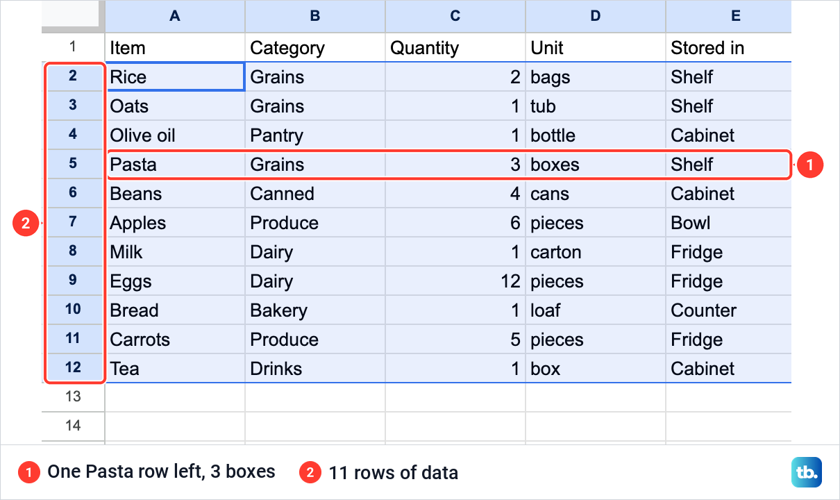
So the boxes you tick decide which columns are compared, while the cleanup works on the range you selected, and with our whole table selected it removed complete rows, never single cells. Select every column of the table before you start. If the rows you would lose hold something you need, tick more columns or use the UNIQUE formula described below instead.
Choose which row is kept
In both of our runs, the first row of each set stayed and the later ones went. That puts you in control: sort the table first so the row you want to keep sits on top. Sort by a date column with the newest first, for example, and a one-column cleanup then keeps the latest entry for each item.
Sort the whole table rather than one column, or the rows will be scrambled. Select the range, choose Data > Sort range > Advanced range sorting options, tick Data has header row there as well if your table has headings, and pick the column and the order.
Highlight duplicates before you remove them
If you would rather see the repeats before deleting anything, a conditional formatting rule colours them. Select the column to check, here A2:A17, and choose Format > Conditional formatting. Under Format cells if, pick Custom formula is and enter this formula.
=COUNTIF($A$2:$A$17,A2)>1Change both ranges to match your column, and keep the dollar signs in the first one. On our list the Rice, Oats, Beans and all three Pasta cells turned green while the rule was still open, and Done saved it. Nothing is deleted, so you can look at each flagged row before you clean up.
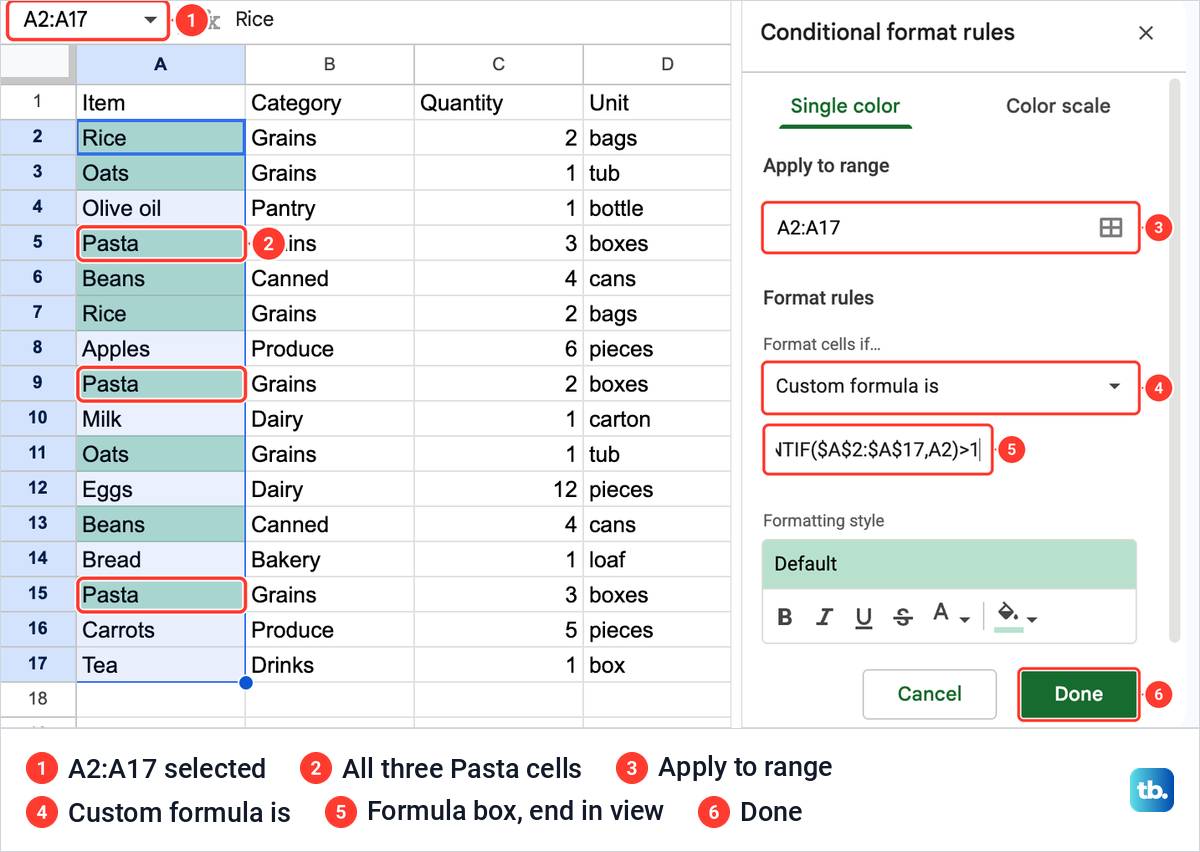
This rule looks at one column only, so it flagged all three Pasta rows, including the 2 boxes row that a full-row cleanup keeps. COUNTIF is not case sensitive, so Rice and rice would light up together.
Keep the original list with the UNIQUE formula
UNIQUE builds a clean copy beside your data, or on another tab, and leaves the original rows alone. Click an empty cell with free space below it and to its right, then type the formula with your table's range. On another tab, include the tab name in the range, as in =UNIQUE('Pantry Items'!A1:E17).
=UNIQUE(A1:E17)We typed it in G1. Sheets filled G1:K13 with the header and 12 distinct rows, the same 12 that Remove duplicates kept, while columns A to E still held all 16 rows. Both Pasta rows appear, because UNIQUE compares whole rows.
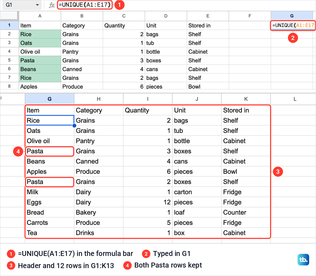
UNIQUE returns rows in the order in which they first appear, so the result follows your list from the top. Because it is a formula, it depends on the source rows, so keep the original table in place while you use the result. To make the result stand on its own, select it, copy it and, with the same cells still selected, press Ctrl + Shift + V, or Cmd + Shift + V on a Mac, to paste values only.
List only the entries that appear once
UNIQUE has a third setting that Remove duplicates has no match for: it drops every copy of a repeated value, including the first. The setting is called exactly_once, and it is off by default. We put the two versions side by side in two empty columns, under the headings One per item and Once only, and typed this formula in the first.
=UNIQUE(A2:A17)In an empty cell of the next column, we typed the version with exactly_once switched on. Each formula goes in its own cell, with empty cells below it for the results.
=UNIQUE(A2:A17,FALSE,TRUE)The first listed 11 item names, one of each. The second listed 7: Olive oil, Apples, Milk, Eggs, Bread, Carrots and Tea. Rice, Oats, Pasta and Beans were left out entirely, because each of them appears more than once.
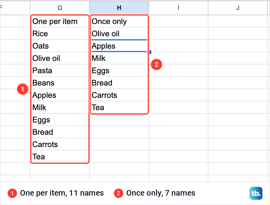
The FALSE in the middle keeps the comparison row by row, which is the default. Use this version to find entries that were only ever recorded once, such as an item bought a single time.
Why some duplicates are not removed
A stray space is the usual cause. We added a row reading Tea, Drinks, 1, box, Cabinet with a space typed before Tea, which looks the same as the other Tea row on screen. Remove duplicates then found 4 duplicates and left 13 rows, so the row with the space was not treated as a copy.
Next we selected the table and ran Data > Data cleanup > Trim whitespace. The message read Trimmed whitespace from the 1 selected cell, and the next Remove duplicates run found 5 duplicates and left 12 rows. Run Trim whitespace first whenever a list came from a form, an export or another app.
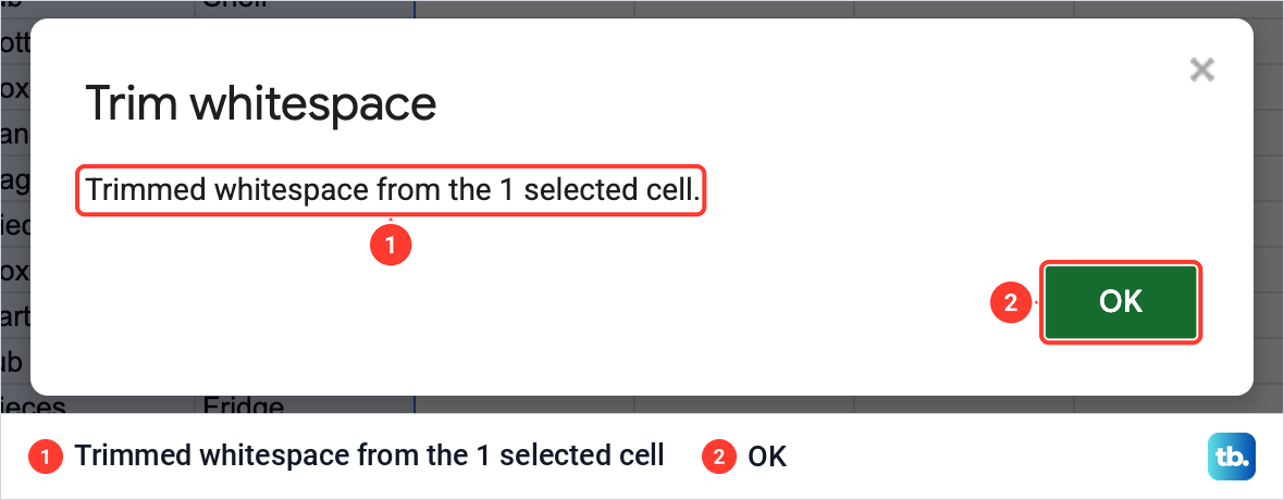
Trim whitespace does not remove non-breaking spaces, which often come along with text pasted from web pages, so a duplicate can survive even after trimming. For UNIQUE, check for hidden text such as trailing spaces, and format numbers the same way, percentages as percentages and currency as currency.
Letter case works the other way for Remove duplicates. That command treats cells with identical values but different letter cases, formatting or formulas as duplicates, so Rice and RICE count as the same item.
Remove duplicates on Android, iPhone and iPad
On a phone or tablet, the cleanup is done in a browser on a computer. To remove duplicates, trim whitespace or split text into columns, open the spreadsheet at sheets.google.com on your computer, sign in with the same Google account and follow the steps in the first section. The file you see there is the same one the Sheets app opens, so the cleaned list shows up on your phone afterwards.
Get removed rows back or work on a copy
If a cleanup removed the wrong rows, undo it at once. On our Mac, Cmd + Z right after the cleanup brought all 16 rows back in one step, and it did the same after each of our runs. On Windows and ChromeOS the shortcut is Ctrl + Z.
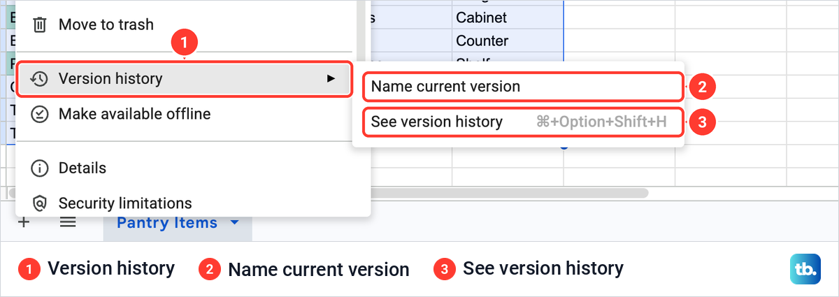
Later on, version history is the way back. Open File > Version history > See version history, pick an earlier time and select Restore this version. You need to own the spreadsheet or have edit access to it.
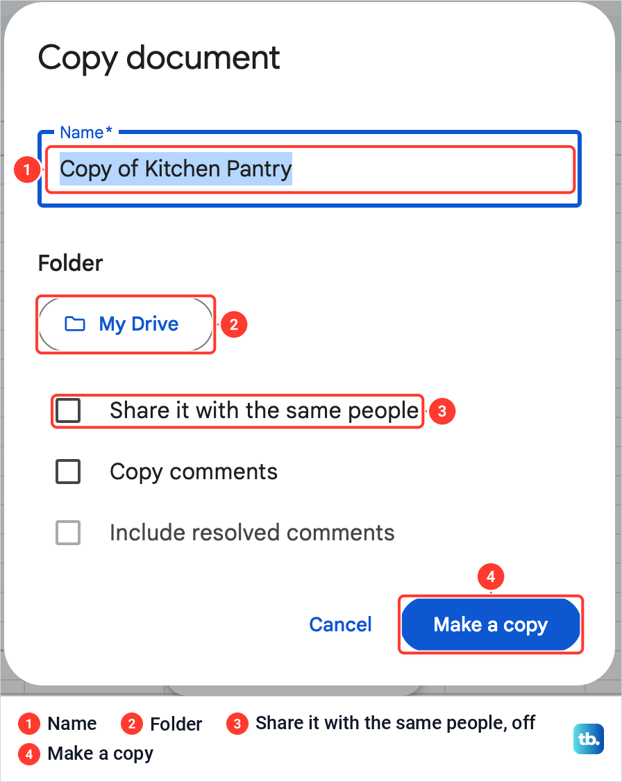
The safest habit is to clean a copy. File > Make a copy opened a Copy document box with Copy of Kitchen Pantry as the name, a folder button set to My Drive, and three boxes that were all unticked, including Share it with the same people. Rename it if you like and select Make a copy, and the copy opens in a new tab.
If your list comes from Excel or goes back to it
Sheets can open an Excel workbook, and File > Download saves a copy you can open in other programs, Excel included. A little preparation on the Excel side makes the cleanup more reliable. If the list reached you as a PDF, convert the PDF to Excel first and open that workbook in Sheets.
Before you bring a workbook across, unhide its hidden columns in Excel so every field is in view when you choose the columns to compare. If one cell holds two facts, such as 3 boxes, split the cells into separate Excel columns first, so you can compare the quantity and the unit on their own.
Lists that people keep adding to will collect duplicates again. If the list goes back to Excel and people keep adding to it there, a drop-down list in Excel keeps entries such as the storage place spelled one way, so the same shelf is not entered as both Cabinet and Cupboard. Once the clean list is back in Excel, alphabetize the rows in Excel if you want it in A to Z order, because Remove duplicates leaves the remaining rows in their original order.
If the clean list goes back to Excel, you can check it there: create a pivot table in Excel that counts each item. After a one-column cleanup every count should be 1, but a name with a stray space shows up as a separate label with its own count, so look for two labels that read the same. If your cleanup compared two columns, such as Item and Unit, combine two columns in Excel into one key first and count that instead.
How we tested this guide
We tested this in Google Sheets on the web in Chrome on a Mac, running Remove duplicates, UNIQUE and a highlight rule on a 16-row pantry list.
Frequently Asked Questions
How do I remove duplicates based on one column in Google Sheets?
Select the whole table, open Data > Data cleanup > Remove duplicates, tick Data has header row if the first row holds column names, untick Select all and tick only that column. Sheets then deletes every later row that repeats a value in that column, including the other fields in those rows.
Does Remove duplicates delete the whole row?
It works on the range you select, so select every column of the table first. With our whole table selected, it removed complete rows and kept the first row of each matching set, and a Pasta row with a different quantity went when only the Item column was compared.
Which duplicate does Google Sheets keep?
The first one, counting from the top of your selection. To keep a different row, such as the newest, sort the whole table so that row comes first before you run the cleanup.
How do I remove duplicates but keep the original data?
Type =UNIQUE(A1:E17) in an empty cell, using your own range, and Sheets lists each distinct row once while the original stays as it is. You can also make a copy of the file with File > Make a copy and clean the copy.
Why are some duplicates still there after Remove duplicates?
Usually a leading or trailing space makes two rows look the same while they differ. Run Data > Data cleanup > Trim whitespace on the table and then Remove duplicates again. Non-breaking spaces, common in text pasted from web pages, are not trimmed.
Can I remove duplicates in the Google Sheets app?
On Android, iPhone and iPad, open the spreadsheet at sheets.google.com on a computer to remove duplicates or trim whitespace. Sign in there with the same Google account and use Data > Data cleanup > Remove duplicates.
How do I get deleted duplicate rows back?
Press Ctrl + Z, or Cmd + Z on a Mac, straight after the cleanup, which brought every row back on our list. Later, use File > Version history > See version history and restore an earlier version, which needs ownership of the file or edit access.