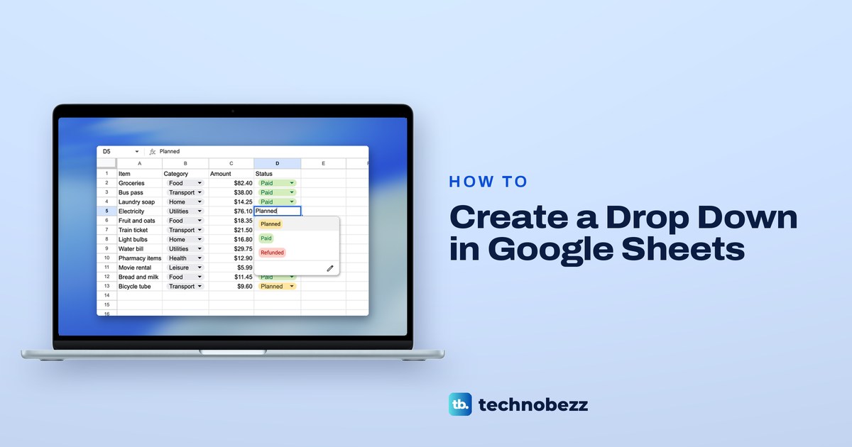
To create a drop-down list in Google Sheets, select the cells that should get the list, click Insert > Dropdown, type your first two choices in the Option 1 and Option 2 fields of the panel that opens, and click Add another item for each choice after that. Click Done, and every selected cell gets an arrow that opens your choices. To take the choices from cells instead, pick Dropdown (from a range) under Criteria.
We built two dropdowns in Chrome on our spending sheet, one typed and one fed from a tab of categories, then changed their source cells, styles and rules. Know three results before you start: renaming a source cell does not change cells that already hold the old word, a range one row short drops the last choice, and Plain text style hides the arrow completely.
The short version
- Typed list: select the cells, click Insert > Dropdown, enter each choice and click Done.
- List from cells: choose Dropdown (from a range) under Criteria and enter a range such as Categories!A2:A7.
- Fill a column fast: type a choice in a dropdown cell and press Enter. The selection moves down a row.
- Allow other words: under Advanced options, switch from Reject the input to Show a warning.
- Phones: the Android app makes lists under More > Data Validation. On iPhone and iPad you can only pick from a list made on a computer.
Ways to add a dropdown at a glance
| Route | Where to find it | Best for |
|---|---|---|
| Insert > Dropdown | Menu bar, with the cells selected | A short typed list such as Planned, Paid, Refunded |
| Data > Data validation > Add rule | Menu bar, then the side panel | Choosing Dropdown (from a range) and seeing every rule on the tab |
| Right-click > Dropdown | The cell menu, near the bottom | Turning words already in the cells into choices |
| Type @, then Dropdowns | Inside an empty cell | Preset lists such as Project status or Priority |
| The pencil at the foot of an open list | Any cell that has a dropdown | Changing a dropdown you already made |
| More > Data Validation | Google Sheets app on Android | Making a list on a phone or tablet |
On our sheet, Insert, Data validation and the pencil all opened the same Data validation rules panel. Right-click > Dropdown on cells that already hold words turns those words into the choices, and typing @ in an empty cell and choosing Dropdowns under components offers the presets.
Create a drop down list with Insert Dropdown
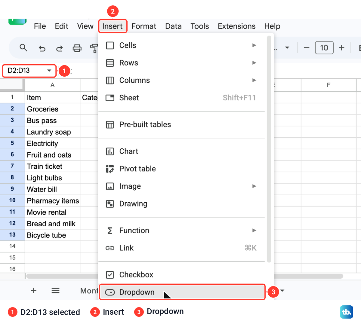
Select the cells that will hold the list. In our spending sheet that was D2:D13, the empty Status column, and the Name box read D2:D13. If your table has no empty column for the list, add a column in Google Sheets first. Then click Insert in the menu bar and choose Dropdown, near the bottom of the menu, right after Checkbox, the entry you use to add check boxes in Google Sheets.
A panel titled Data validation rules opens on the right. Apply to range holds the cells you selected, Criteria is set to Dropdown, and there are two empty fields, Option 1 and Option 2. The moment it opened, every cell in D2:D13 showed an empty grey chip with an arrow, before we had typed a single choice.
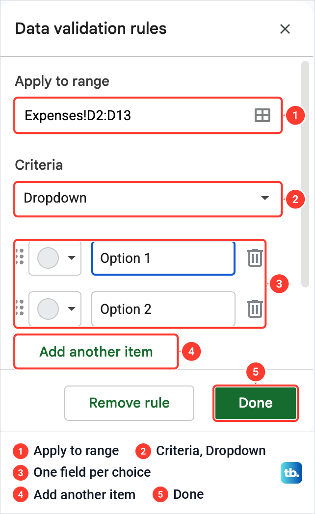
Type your first choice in Option 1 and the second in Option 2. Click Add another item for each extra choice: we typed Planned and Paid, added a third field and typed Refunded. Each choice has a color button and a bin, and under the list sits an unticked box named Allow multiple selections.
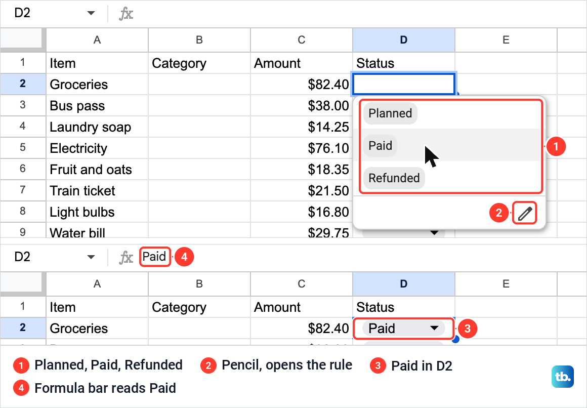
Click Done, and the panel turns into a list of the tab's rules, where ours read Value contains one from list, with D2:D13 under it. Click any cell in the range and its list opens with your choices and a small pencil at the bottom right. We clicked D2 and picked Paid. The cell showed a Paid chip and the formula bar read Paid, so the cell stores the word itself.
Make a dropdown from a range of cells
A typed list lives inside the rule. When the choices are already in cells, point the dropdown at those cells instead. Our spending sheet keeps six categories on a tab named Categories, in A2:A7: Food, Transport, Home, Utilities, Health and Leisure.
The list shows the choices in the same order as those cells, so sort the source cells alphabetically first if you want them from A to Z. If you are collecting the words from a column you already filled in, remove duplicates in Google Sheets so each category appears once in the source.
Select the cells that get the list, B2:B13 in our case, and click Data > Data validation, then Add rule. Open the Criteria box, where Dropdown (from a range) sits second, above rules such as Text contains. Choose it and type the source range with its tab name, such as Categories!A2:A7.
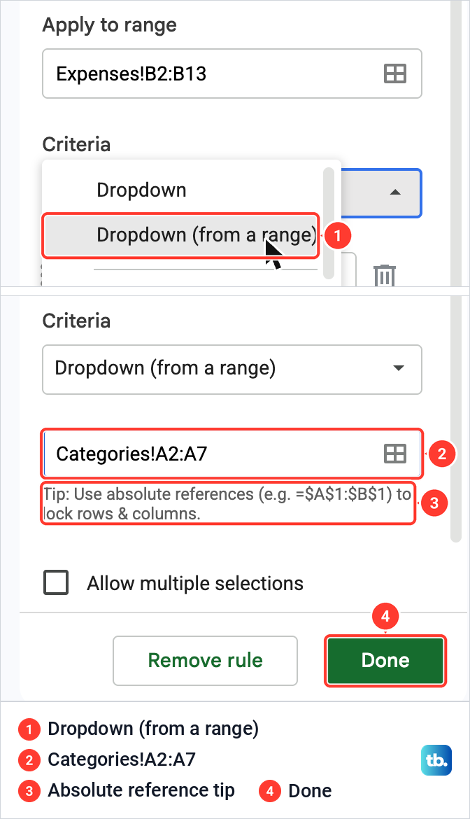
Sheets shows a tip under the field about absolute references, but you do not have to type the dollar signs yourself. When we reopened a rule we had typed as Categories!A2:A6, the field read =Categories!$A$2:$A$6, and the choices it found were listed underneath, each with its own color button.
Click Done. Every cell in B2:B13 now opens the six categories, and the list in B11, near the bottom of the table, opened upward instead of down. The side panel then listed both rules on the tab, one for B2:B13 and one for D2:D13.
What happens when the source cells change
A dropdown from a range follows its cells. We set B11 to Leisure, then renamed Categories!A7 from Leisure to Entertainment. The next time we opened the list in B2, it offered Entertainment in place of Leisure, with nothing to change in the rule.
The cell that already said Leisure did not change. B11 kept its word and gained a small red triangle in its top right corner, and resting the pointer on it showed Invalid: Input must fall within specified range. When we put A7 back to Leisure, the mark went away.
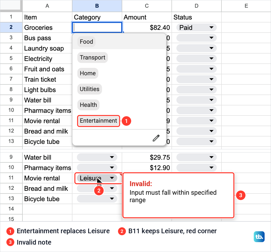
So renaming a choice in the source does not rename it in your data. Look down the column for red corners afterward and pick the new word in each of those cells.
The range also has to cover every choice. On an empty cell beside the table, we made a list from Categories!A2:A6, one row short, and it offered five categories. Leisure, in A7, was missing from the list, and changing the range to A2:A7 brought it back.
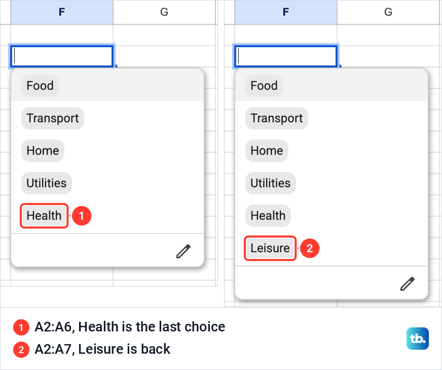
A word you add below the range stays out of the list in the same way, so add new choices inside the range instead. On the Categories tab we right-clicked row number 7, chose Insert 1 row above (the same menu you use to insert multiple rows in Google Sheets) and typed Pets in the new cell. Every Category list offered seven choices straight away, and the rule's range had grown to =Categories!$A$2:$A$8 without us opening it.
Add colors and pick a display style
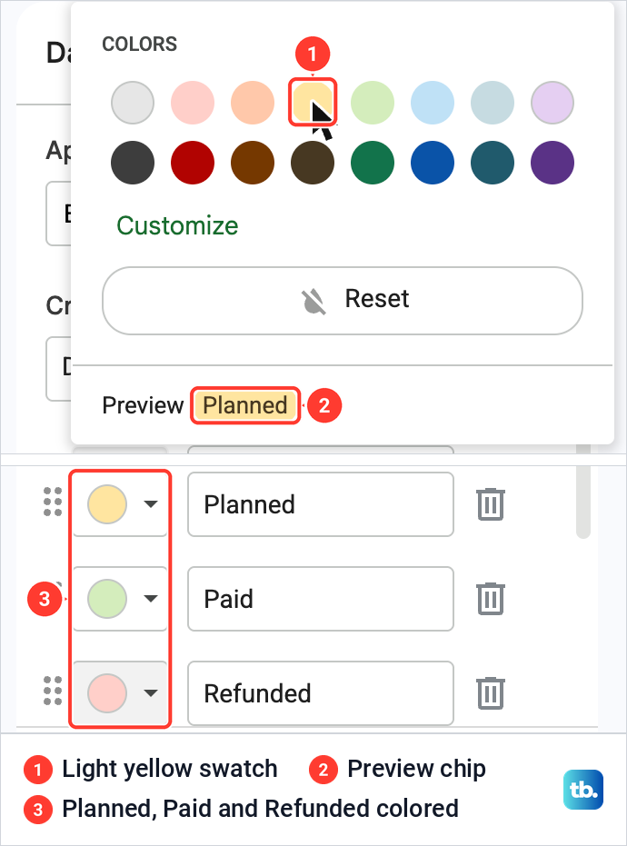
Each choice can have its own color. In the rule, click the color button beside a choice to open a grid of swatches under COLORS, with Customize, Reset and a Preview chip that shows the result. We gave Planned light yellow, Paid light green and Refunded light red, and the colors then showed in the chips and in the open list.
Under the choices, Advanced options holds three more settings: Show help text for a selected cell, If the data is invalid, and Display style. Our new rule came with Reject the input and Chip selected by default, and the help text box unticked.
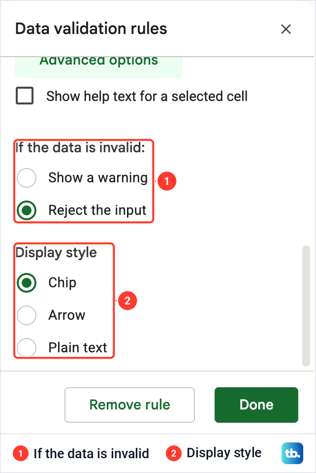
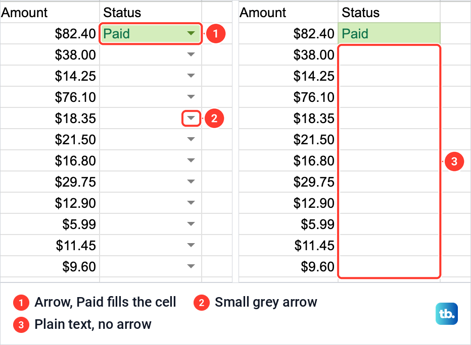
Display style mainly changes how the dropdown looks, but keep Chip if you want to allow multiple selections. Chip is the rounded pill with an arrow. Arrow drops the pill and puts a small grey arrow at the right of the cell, and a colored choice then fills the whole cell, as our green Paid did in D2.
Plain text hides the dropdown completely: no arrow and no pill, so an empty cell with a list looks like any other empty cell. The list still works, and selecting the cell and pressing Enter, or starting to type, opened the three choices under it as plain words. The change showed in the sheet as soon as we clicked a style, before Done.
Allow more than one choice in a cell
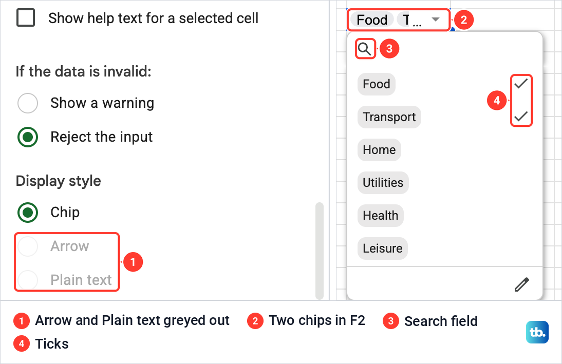
Tick Allow multiple selections in the rule to let one cell hold several choices. It works only with the Chip style. With the box ticked, Arrow and Plain text went grey under Display style, and while the style was Plain text, the tick box itself was greyed out.
We tried it on an empty cell beside the table, using the same category range as column B. When we clicked Done, Sheets asked "Apply to all? There are 12 other dropdowns with the same properties, do you want to make changes to all of them?" We chose Just this instance to change only this cell. Apply to all, as the question says, would change the 12 matching dropdowns too.
The list then had a search field, stayed open after each pick and ticked each chosen item. We picked Food and Transport, and the cell showed two chips.
Two more limits apply. Remove any spaces at the start or end of a choice, because they stop multiple selections from working. In the Android and iPhone apps you cannot select more than one choice yet, even when the rule allows it.
Choose what happens to other entries
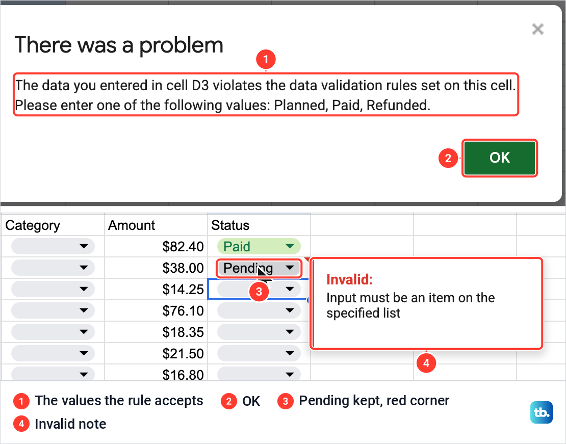
A dropdown cell still accepts typing, so the rule decides what happens to a word not on the list. With Reject the input, the setting our rule came with, we typed Pending in D3 and pressed Enter. A box titled "There was a problem" appeared, and after OK the cell was still empty.
The message reads: "The data you entered in cell D3 violates the data validation rules set on this cell. Please enter one of the following values: Planned, Paid, Refunded." It names the cell and every allowed value.
To let other words in, open the rule, click Advanced options and select Show a warning. We typed Pending again, and this time it stayed, as a grey chip with a red triangle in the corner. Resting the pointer on it showed Invalid: Input must be an item on the specified list.
Show a warning suits a list you expect to grow, because nobody is blocked and the red corners show what to tidy up later. Switching back to Reject the input does not clean up afterward. When we did, the Pending already in D3 stayed where it was.
Edit, clear or remove a dropdown
To change a dropdown, click one of its cells to open the list, then click the pencil at the bottom right. Its tooltip reads Edit button, and it opens that cell's rule in the side panel.
To add a choice, click Add another item, type it and click Done. We added Pending as a fourth choice, with a grey color button. It appeared in the list, and the Pending already in D3 lost its red corner, because it was now a valid choice.
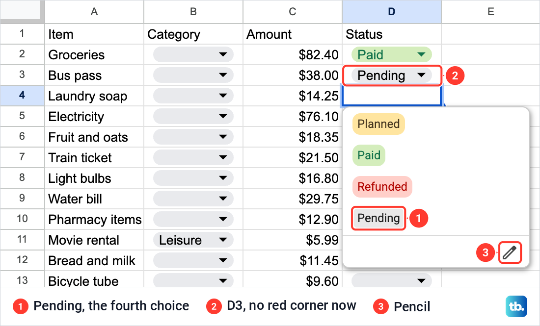
Deleting a choice works the other way round. When we removed Pending with its bin, the change applied at once, before we clicked Done, and the red corner came back on D3. Cells keep whatever they hold when a choice disappears.
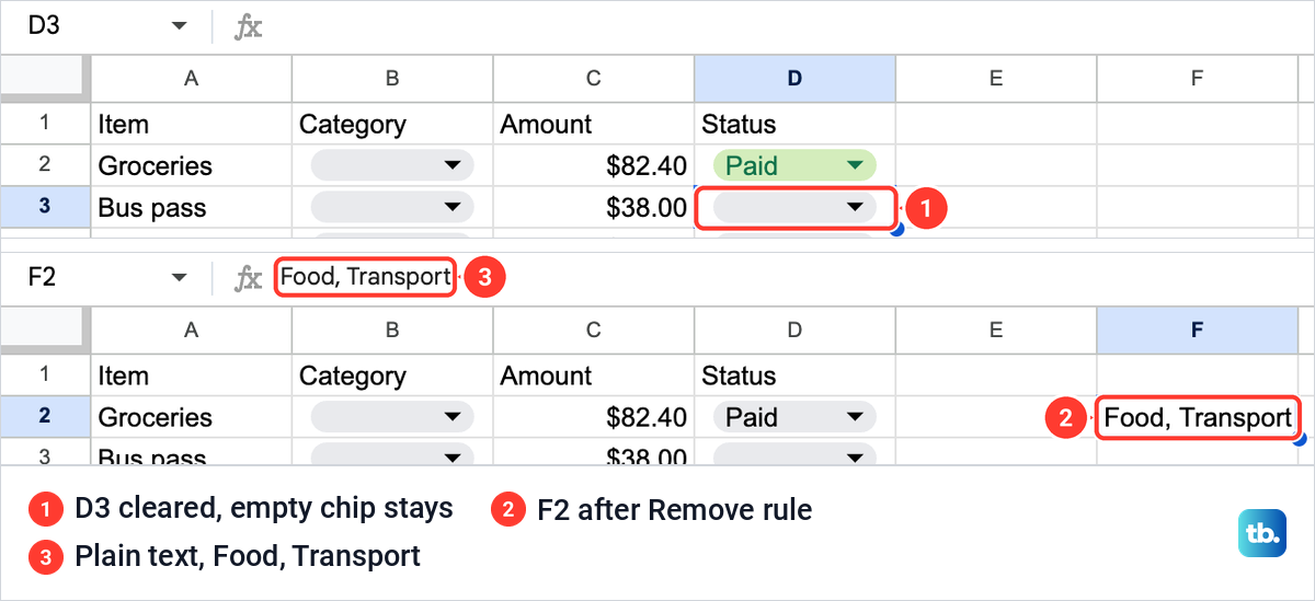
Clearing a cell and removing the dropdown are different things. Select a cell and press Delete once, and only the word goes: when we cleared D3, the empty chip and its arrow stayed, ready for a new pick. On cells that are already empty, Backspace (the delete key on a Mac) removes the dropdown itself. To take the dropdown off any cells, open the rule and click Remove rule.
Remove rule does not ask for confirmation, and it does not wipe the cells. On our multi-select cell it removed the dropdown and left Food, Transport in the cell as plain text.
Fill a column quickly and fit long choices
Clicking each arrow gets slow on a long column, so type instead, and freeze a row in Google Sheets first so the headings stay in view. With a dropdown cell selected, type the choice and the list narrows as you go. Press Enter to take it, and the selection moves down to the next cell. We filled the twelve cells of our Category column this way.
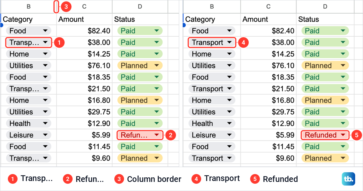
Long choices get cut at the default column width. Our chips read "Transp..." and "Refun..." until we double-clicked the right border of the B and D column letters. Each column then fitted its widest entry, and every chip showed its whole word.
With one spelling for each category, you can total a column in Google Sheets by category. You can make a graph in Google Sheets from them, with no stray spelling splitting a category in two.
Create a dropdown in the Android app
The Google Sheets app for Android can make and edit dropdowns, but its labels differ from the web. Open the spreadsheet, tap the cells for the list, tap More at the top right and tap Data Validation. Under Criteria, choose List of items, or choose List from a range and enter the cells.
For each choice in a list of items, tap +Add, enter the item and tap Done. Tap Save at the top right when the list is complete. On Android, a word outside the list gets a warning by default, so choose Reject input under On invalid data if only listed words should go in. Turning off the Show dropdown list in cell switch removes the arrow from the cells.
To change a list, take the same path, edit the items under Criteria and tap Save. To delete it, tap Remove rule at the bottom right.
Use a dropdown on iPhone or iPad
The Sheets app on iPhone and iPad cannot create or edit a dropdown, so make the list in a browser on a computer first. Once it exists, open the spreadsheet in the app, tap a cell with a dropdown and pick a choice. Only one choice can be picked there, even in a cell that allows several, and any change to the choices has to be made back on a computer.
When a dropdown list does not behave
Most dropdown trouble comes down to the rule's range, its source or its settings. Open the rule from the pencil and read Apply to range first, because a cell outside it has no list at all. Then check the source field of a list from a range. A red corner means the cell holds a word the current list does not allow, either because the source changed or because someone typed another word under Show a warning.
How we tested this guide
We tested this in Google Sheets on the web in Chrome on a Mac, adding dropdowns to two columns of a 12-row household spending sheet and changing their rules.
Frequently Asked Questions
How do I make a dropdown in Google Sheets quickly?
Select the cells, click Insert > Dropdown, type each choice and click Done. Use Add another item for every choice after the second.
Does a Google Sheets dropdown update when I change its list?
A list made with Dropdown (from a range) follows its source cells, so a renamed word inside the range shows up in the list straight away. Cells that already hold the old word keep it and get a red corner, so pick the new word in those cells yourself.
How do I let people enter a value that is not on the list?
Open the rule, click Advanced options and choose Show a warning under If the data is invalid. The word is then kept with a red corner instead of being refused.
Can I select more than one option in a dropdown cell?
Yes, on a computer. Tick Allow multiple selections in the rule, which works only with the Chip display style. The Android and iPhone apps cannot pick more than one choice yet.
Can I create a dropdown in the Google Sheets app on iPhone?
No. Create and edit dropdowns on a computer, and the iPhone and iPad app can then pick a choice from them. The Android app can create them under More > Data Validation.
How do I remove a dropdown but keep the text?
Open the rule with the pencil at the foot of its list and click Remove rule. The dropdown goes, and whatever the cells held stays as plain text.