To hide a row in Google Sheets, right-click its row number and choose Hide row, and to hide a column, right-click its letter and choose Hide column. To unhide them, click one of the small arrows that appear where the row number or column letter used to be, or select the rows on both sides of the gap, right-click and choose Unhide rows.
We hid and brought back single rows, a block of rows and a column in our Weekly expenses sheet in Chrome. When you select several rows, the right-click menu names the range it is about to hide, and one Unhide rows command brought back two separate hidden blocks at once.
The short version
- Right-click a row number and choose Hide row, or right-click a column letter and choose Hide column.
- Select several row numbers first to hide a whole block in one go.
- Click an arrow at the gap to show a row or column again, or select across the gap and choose Unhide rows.
- On Windows, Ctrl + Alt + 9 hides rows and Ctrl + Shift + 9 unhides them; use 0 for columns.
- Numbers missing but no arrows? A filter or a collapsed group is hiding those rows.
Hide a row in Google Sheets
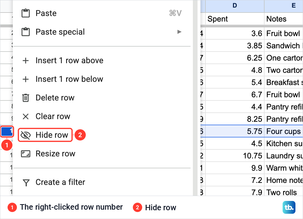
Find the row you want to hide and look at its number in the grey strip on the left. Right-click that number, and a menu for the whole row opens. Choose Hide row.
We right-clicked the number of row 10 in our Weekly expenses sheet, the Yogurt line. Hide row sits between Clear row and Resize row, and Delete row is only two lines above it, so read the label before you click.
The row disappeared from view, and the numbers on the left now ran 9 and then 11. A small arrow showed beside each of those two numbers, pointing up at 9 and down at 11. Nothing else in the sheet moved or changed.
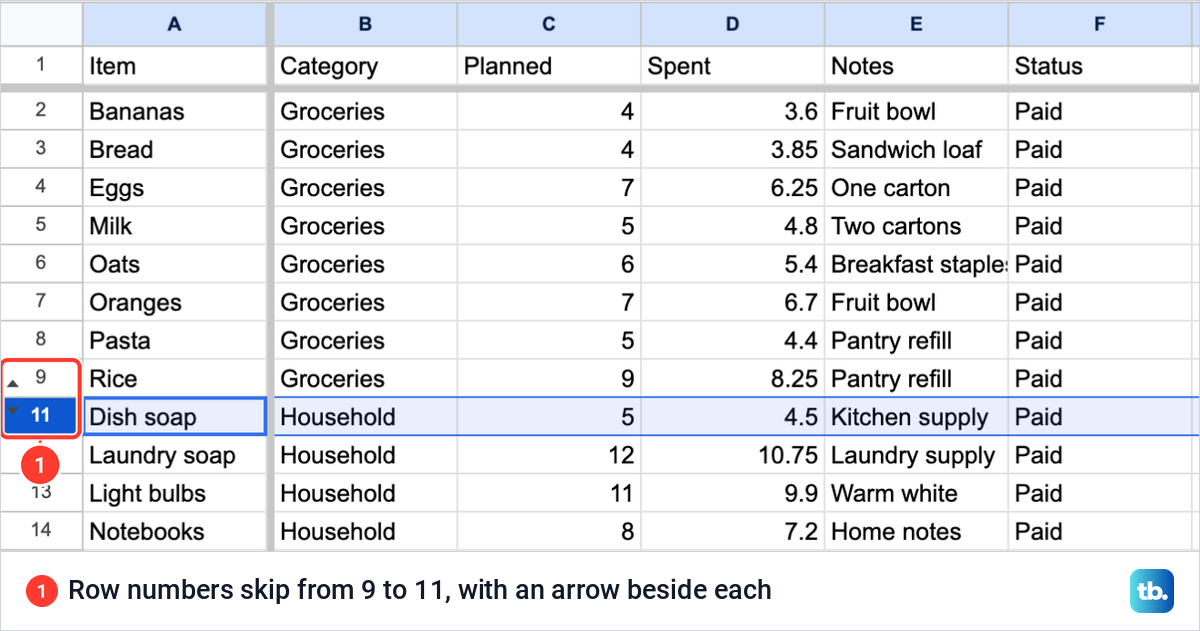
The thick grey lines under row 1 and beside column A in our pictures are not hidden rows. They mark a frozen heading row and a frozen Item column, which stay on screen while you scroll. A hidden row shows up as a gap in the numbers instead.
Hide several rows at once
To hide a block of rows, select them all first. If the rows you want out of the way are scattered through the table, sort the sheet by the column they share so they sit together.
Click the first row number, hold Shift and click the last one, or drag down the numbers, then right-click anywhere on the blue numbers. We selected rows 5 to 7, and the menu changed to name the range, with Hide rows 5 - 7 under Delete rows 5 - 7 and Clear rows 5 - 7.
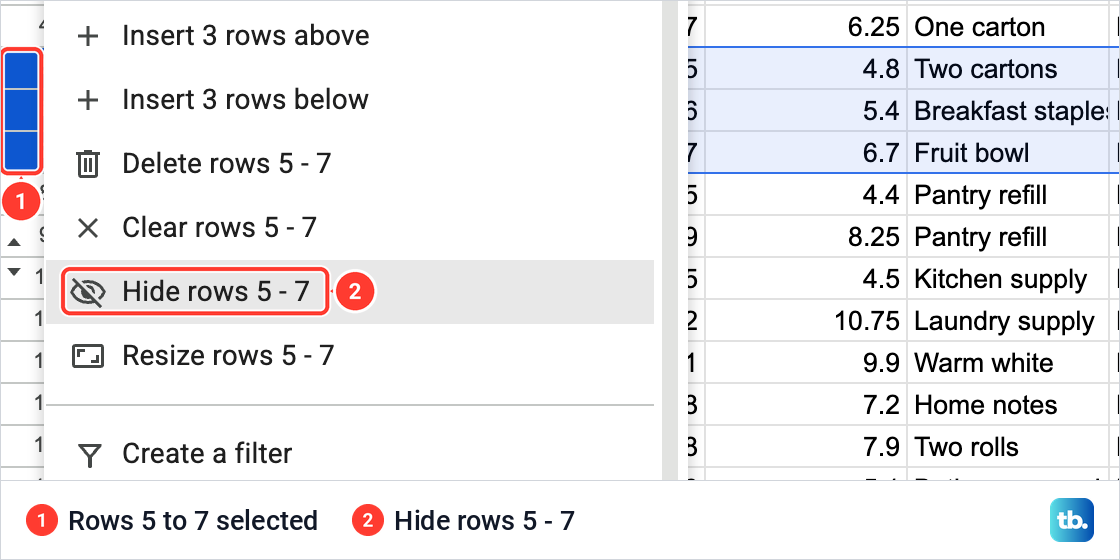
That label is a useful last check. If it names rows you did not mean to touch, close the menu and fix the selection before you choose anything. Each block you hide gets its own pair of arrows, so two hidden blocks show two gaps in the numbers.
For rows that are not next to each other, hold the Command key on a Mac, or Ctrl on Windows, while you click each row number. Then right-click one of the blue numbers and choose the hide command.
Unhide rows in Google Sheets
To show a hidden row again, click one of the small arrows beside the row numbers on either side of the gap, where the missing number used to be. The row returns to its place. The arrows are small, so zoom the page in if they are hard to hit.
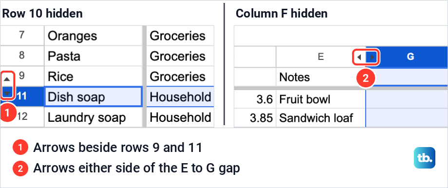
The other way is the right-click menu, and it can clear several gaps at once. With rows 5 to 7 and row 10 hidden, we selected rows 4 to 11, which spans both gaps, and right-clicked the row numbers. The menu gained an extra entry, Unhide rows, just under Hide rows 4 - 11.
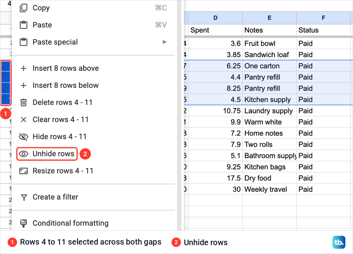
Choosing Unhide rows brought back rows 5, 6, 7 and 10 in one go. The other labels in that menu counted the hidden rows too. It offered to insert 8 rows, the entry you use to insert multiple rows in Google Sheets, and named Delete rows 4 - 11, a range that includes the rows you cannot see.
To bring back every hidden row in a sheet, including a hidden row 1 or last row, select the whole sheet with Ctrl + A (Command + A on a Mac). Check that the whole grid is selected and not only your table, then press Ctrl + Shift + 9 (Command + Shift + 9) to unhide the rows.
Hide and unhide columns
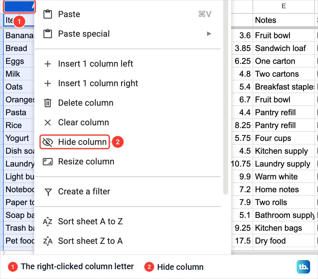
Columns work the same way from the letters along the top. Right-click a column letter and choose Hide column, which sits between Clear column and Resize column. Just above them, Insert 1 column left and Insert 1 column right are the entries you use to add columns in Google Sheets.
We hid column F, the Status column. The letters at the top then ran E and then G, with a small arrow on each side of the gap, and the Status values were out of view. Click either arrow to bring the column back.
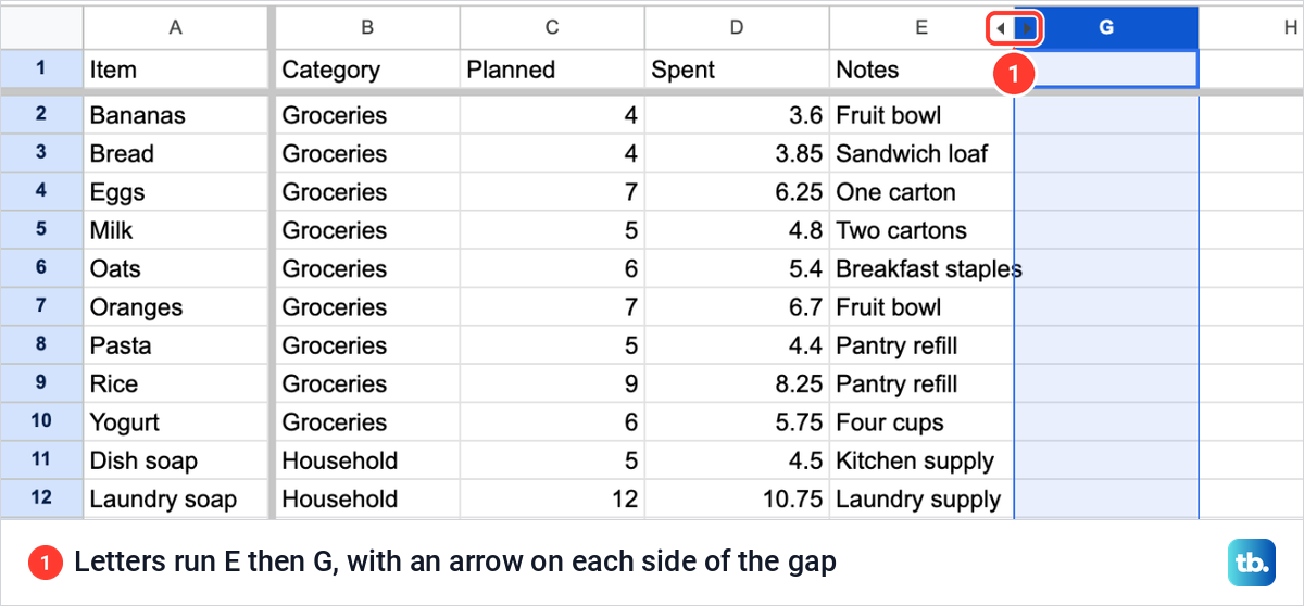
The menu route works for columns too. We selected columns E to G, the two columns either side of the gap, and right-clicked the letters. Next to Hide columns E - G, the menu offered Unhide columns, and choosing it put column F back.
To hide several columns at once, select their letters first by dragging across them or with Shift. The menu entry then becomes Hide columns with the range in its name.
Keyboard shortcuts to hide rows and columns
Sheets has a shortcut for each of the four jobs. Select the row or column first by clicking its number or letter, then press the keys. To unhide, select the rows or columns on both sides of the gap before you press the unhide keys.
| What you want | Windows and ChromeOS | Mac | Without the keyboard |
|---|---|---|---|
| Hide rows | Ctrl + Alt + 9 | Command + Option + 9 | Right-click the row numbers, then Hide row |
| Unhide rows | Ctrl + Shift + 9 | Command + Shift + 9 | Click an arrow at the gap, or select across it and choose Unhide rows |
| Hide columns | Ctrl + Alt + 0 | Command + Option + 0 | Right-click the column letters, then Hide column |
| Unhide columns | Ctrl + Shift + 0 | Command + Shift + 0 | Click an arrow at the gap, or select both sides and choose Unhide columns |
Some shortcuts do not work with every language or keyboard layout. If a combination does nothing, the right-click menu has the same commands, and Ctrl + / on Windows or Command + / on a Mac opens the list of shortcuts inside Sheets.
Rows missing but no arrows to click
A gap in the row numbers with no small arrows means the rows were not hidden with Hide row. The two usual causes are a filter and a collapsed group, and each one has its own control.
A filter hides rows by their values. Look for the small filter buttons in the heading row, open the one for the column that is filtered and tick the values you want to see again. To switch the filter off completely, choose Data > Remove filter. Anyone with access to the file sees a filter too, so a filter left on hides those rows for everyone.
A group folds rows away behind a small control beside the row numbers. Click Plus (+) to expand the rows and Minus (-) to collapse them again. To remove the group itself, select its rows and choose View > Group > Ungroup rows.
If a whole tab is missing rather than some rows, the sheet itself is hidden. Open the View menu and look for Hidden sheets, then choose the sheet's name.
What hidden rows do to totals
If you total a column in Google Sheets with a plain SUM, the total still includes hidden rows in its range. It keeps adding every cell whether the row is on screen or not, so hiding a row does not change that total.
To add only the rows you can see, use Google's SUBTOTAL function with a code that skips hidden rows. On our sheet the Spent amounts sit in D2 to D19, so the formula below goes in an empty cell under them.
=SUBTOTAL(109, D2:D19)Code 109 adds the visible cells and skips the rows you hid by hand, while code 9 counts them too. Rows hidden by a filter are never included in SUBTOTAL, whichever code you use.
Hidden rows can also get in the way of a filter. Hidden rows or columns are among the reasons Create a filter can be unavailable, and the fix is to unhide them and try again.
A chart drawn from the same rows changes too. In a spending sheet with a pie chart, we hid one of the three rows the chart reads, and the pie redrew at once with two slices instead of three. Sheets showed the note Data in hidden rows is excluded from the chart with an Include data link beside it, and unhiding the row brought the third slice back. Our guide shows how to make a graph in Google Sheets.
Hidden rows and columns are not private
Hiding is for a tidier view, not for secrets. Anyone who can edit the file can click the arrows, and even viewers who make a copy can unhide hidden sheets, so treat a hidden row or column as visible to everyone you share the file with.
If someone should not see a column at all, keep it in a separate file you do not share. If they only need the visible part, hide the column and take a screenshot on any device instead of sending the file.
To stop people changing cells rather than seeing them, Data > Protect sheets and ranges limits who can edit. Protection is not a security measure either, because people can still copy, print and export a protected spreadsheet.
To clear rows out of your own way without changing what others see, use a filter view. A filter view made with Data > Create filter view on a computer applies only to your view of the spreadsheet.
Filter rows by a value instead
A formula cannot hide a row by itself, so rows do not vanish when a cell changes. The closest built-in way is a filter on a column such as Status that leaves out a value like Paid, and you change the filter when you want the rows back.
If you filter by a specific Status value, spell that value the same way every time. A Status column filled from a drop-down list in Google Sheets keeps the spelling consistent, and the column menu in Sheets has a Dropdown entry for this.
For a rule you want to spell out in a formula, add a helper column with an IF formula that returns Hide or Show, then filter that column. One example is =IF(F2="Paid","Hide","Show").
Hide rows in the Google Sheets app on Android
In the Android app, open the spreadsheet, touch and hold a row number or column letter, and tap Hide Row or Hide column in the menu that appears. To group rows instead, highlight them, touch and hold, tap More and then Group.
On a computer, one click on the arrow at the gap brings a hidden row back. With an external keyboard plugged into an Android phone or tablet, Ctrl + Shift + 9 unhides rows and Ctrl + Shift + 0 unhides columns.
Hide rows on an iPhone or iPad
The iPhone and iPad app uses a tap rather than a long press. Open the spreadsheet in the Sheets app, tap a row number or column letter, then tap the right arrow in the menu that appears and choose Hide row or Hide column.
If your menu does not match those steps, update the Sheets app and look again. Hidden rows are saved in the file itself, so rows you hide on the phone can be brought back with the arrows on a computer.
How we tested this guide
We tested this in Google Sheets on the web in Chrome on a Mac, hiding and unhiding single rows, a block of rows and a column in an 18-row expenses sheet.
Frequently Asked Questions
How do I unhide one row in Google Sheets?
Click one of the small arrows beside the row numbers on either side of the gap. You can also select the rows above and below the gap, right-click the row numbers and choose Unhide rows.
How do I unhide all rows at once?
Select the whole sheet with Ctrl + A, or Command + A on a Mac, and check that the whole grid is selected and not only your table. Then press Ctrl + Shift + 9, or Command + Shift + 9. For hidden rows inside your table, selecting from the row above the first gap to the row below the last one and choosing Unhide rows also works.
Why are some row numbers missing with no arrows?
The rows are filtered or grouped, not hidden. Turn the filter off with Data > Remove filter, or click the plus sign beside the row numbers to expand a group.
Can I hide rows only for myself?
Not with Hide row, which changes the view for everyone. Use Data > Create filter view on a computer instead, since a filter view applies only to your view.
Do hidden rows still count in a SUM?
Yes. SUM adds every cell in its range, hidden or not. Use =SUBTOTAL(109, range) to add only the rows you can see.
Does hiding a column keep it secret?
No. Anyone who can edit the file can unhide it in one click. Keep private data in a separate file that you do not share.
How do I hide a row on my phone?
On Android, touch and hold the row number and tap Hide Row. On an iPhone or iPad, tap the row number, tap the right arrow in the menu and choose Hide row.