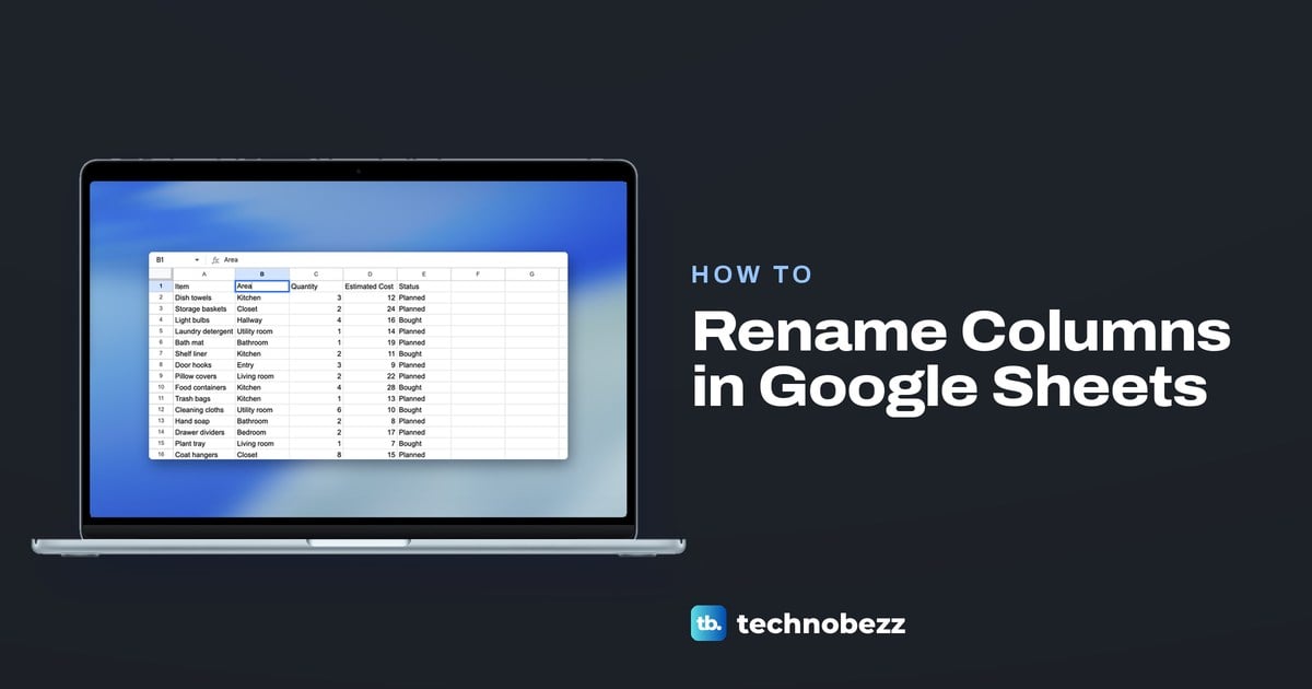
To rename a column in Google Sheets, double-click its heading cell in row 1, such as B1, type the new name and press Enter. The letters above the grid, A, B, C and so on, cannot be renamed: right-click one and the menu has no Rename entry at all. What a reader sees as the column's name is the text in that first cell, so a list that starts in row 1 needs a heading row first.
We renamed the headings of our Household Purchases sheet in Chrome, after giving the list the heading row it lacked. We also checked what a new name does to a table formula, a named range and the sort dialog.
The short version
- Rename a heading: double-click its cell in row 1, type the new name and press Enter.
- The letters stay: A, B and C are cell addresses, and no menu renames them.
- No heading row yet: right-click the row number 1, choose Insert 1 row above and type the names.
- Keep the names in view: choose View > Freeze > 1 row.
- Names in formulas: in a table, our formula followed the renamed heading; a named range gives the cells a name and leaves the heading as it is.
- On a phone: double-tap the heading cell, type the name and tap Done.
What you can rename in Google Sheets
| What you want to rename | Where to do it | What changes |
|---|---|---|
| A column's visible name | Double-click its cell in row 1, type, press Enter | The text in that cell, not the letter |
| A column letter such as B | Nowhere, no menu offers it | Nothing, the letters are fixed cell addresses |
| A table column | Double-click the heading inside the table | The heading, and our formula that named it |
| A set of cells for formulas | Data > Named ranges | A name such as planned_costs, not the heading |
| The tab at the bottom | Right-click the tab, then Rename | The sheet's name only |
| The whole file | File > Rename | The spreadsheet's name only |
The table describes Google Sheets on the web. In the phone apps, double-tap a heading cell to change it; the steps are further down.
How to rename a column heading
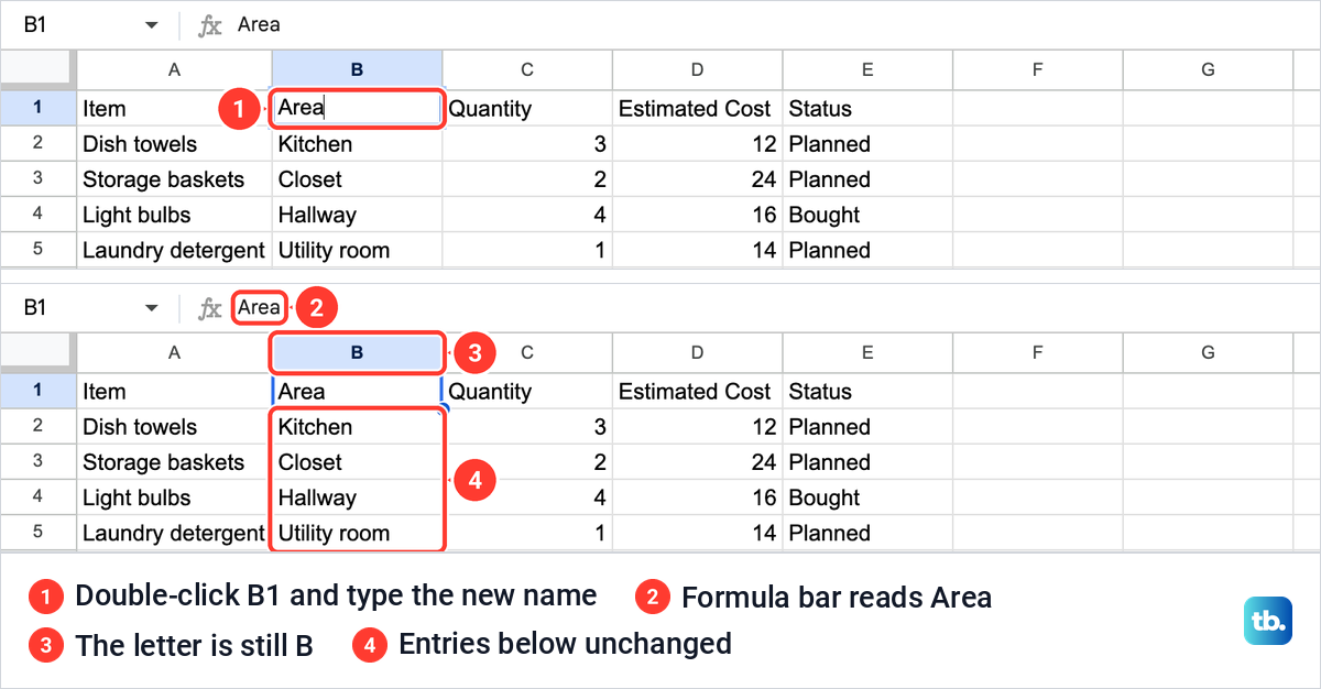
Find the cell in row 1 at the top of the column, B1 for column B. Double-click it, and the cell opens for editing with a cursor in the text. Replace the old name with the new one and press Enter.
In our sheet we double-clicked B1 and replaced Category with Area. While we typed, and after we pressed Enter, the letter above the column still read B and the formula bar read Area. The fifteen entries below it, from Kitchen and Closet down to the last one, did not change.
Repeat this for any other heading. A column's name is only the text in its top cell, so you can change it as often as you like, the same way as any other entry.
Why the column letters cannot be renamed
The letter is the obvious place to look. A right-click on the letter B selected the whole column, and the Name box at the left of the formula bar read B:B. The menu opened with Cut, Copy and Paste, then entries to insert, delete, clear, hide and resize the column.
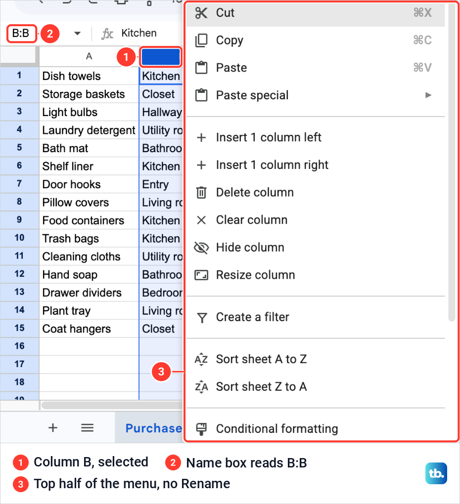
Lower down came the filter, sort and formatting entries, then Data validation, Column stats, Dropdown and Smart chips, with no Rename entry anywhere. The insert entries add a column rather than name one, as our guide to adding columns in Google Sheets shows.
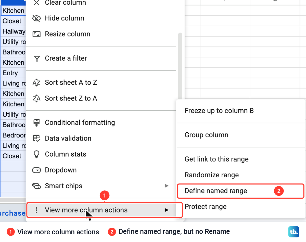
The last entry, View more column actions, opens Freeze up to column B, Group column, Get link to this range, Randomize range, Define named range and Protect range. Still no Rename. The letters are the sheet's cell addresses, the B in B1 and B2, and they stay A, B, C whatever you type into the cells.
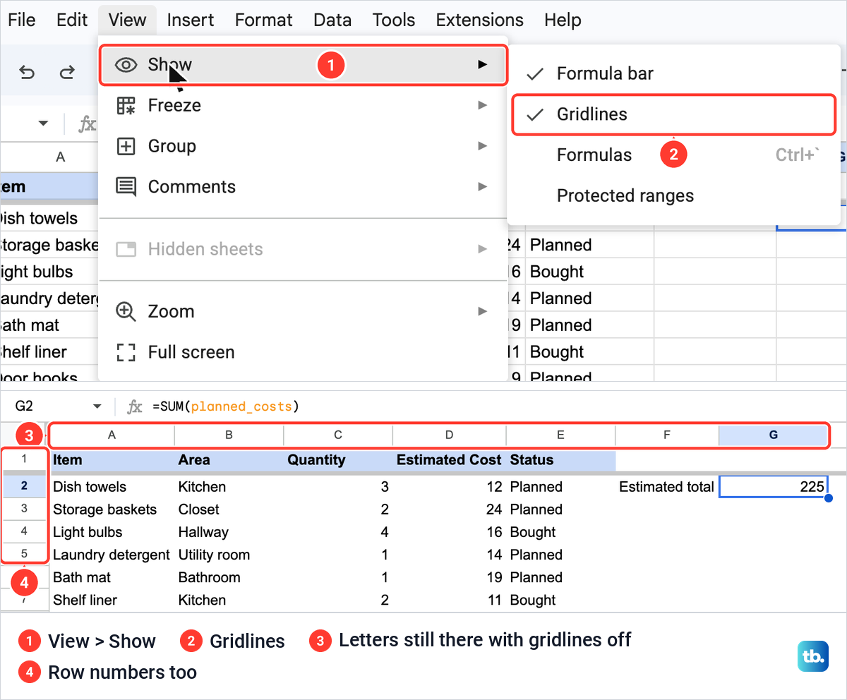
Turning the gridlines off does not hide the letters either. View > Show lists Formula bar, Gridlines, Formulas and Protected ranges, with no entry for the letters. With Gridlines unticked, our sheet lost its grey cell lines, but the letters A to G and the row numbers were still there.
Add a heading row when the list starts in row 1
If your entries begin in the very first row, there is no cell to hold a name yet. Ours did, with Dish towels, Kitchen, 3, 12 and Planned in row 1, straight under the letters. Right-click the row number 1 at the left edge, and the menu offers Insert 1 row above and Insert 1 row below.
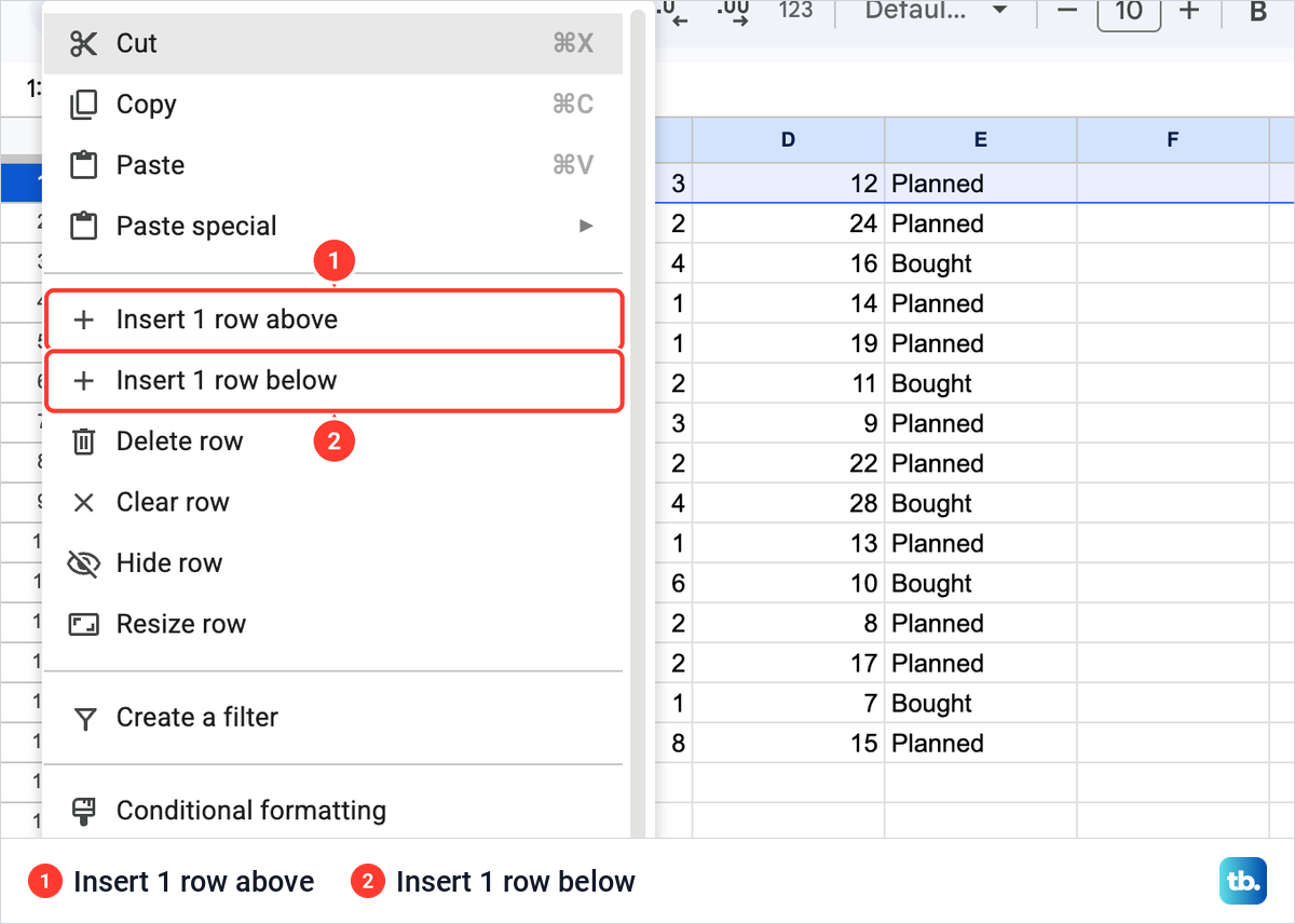
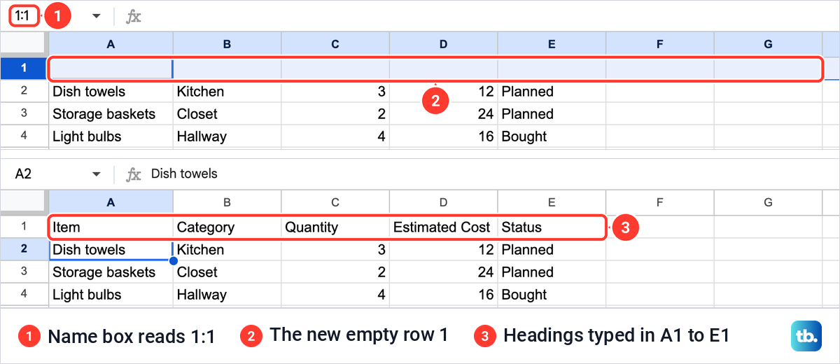
Choose Insert 1 row above. An empty row 1 appeared, already selected with the Name box reading 1:1, and the fifteen entries moved down to rows 2 to 16 unchanged. To add more than one row at the top, select that many row numbers first, as our guide to inserting multiple rows in Google Sheets shows.
Click A1, type the first name and press Tab to move to the next cell along. We typed Item, Category, Quantity, Estimated Cost and Status into A1 to E1, the cells you rename later with a double-click.
Make the headings stand out and stay in view
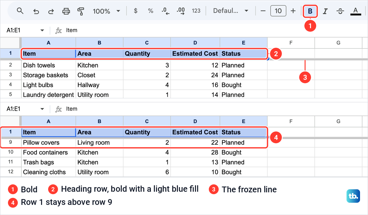
A heading row reads better when it looks different from the data. Select it, A1 to E1 in our case, click Bold in the toolbar and pick a color from Fill color. We used a light blue fill.
In bold, Estimated Cost no longer fitted column D. A double-click on the edge between the letters D and E widened the column to fit it. If you would rather keep a long heading in a narrow column, wrap text in Google Sheets so it runs onto a second line.
To keep the names on screen while you scroll, open View > Freeze. The list offers No rows, 1 row, 2 rows and Up to row 1, then the same for columns, where Up to column E followed our selection. Choose 1 row.
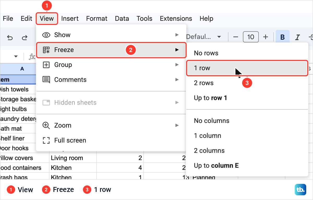
A thick grey bar appeared under row 1. When we scrolled down, the headings stayed in place directly above row 9 while rows 2 to 8 went out of view. Our guide to freezing a row in Google Sheets covers unfreezing and freezing more than one row.
Row 1 matters for charts too. When you make a graph in Google Sheets, the end of the chart editor's Setup tab has a box named Use row 1 as headers.
Make the sort dialog use your heading names
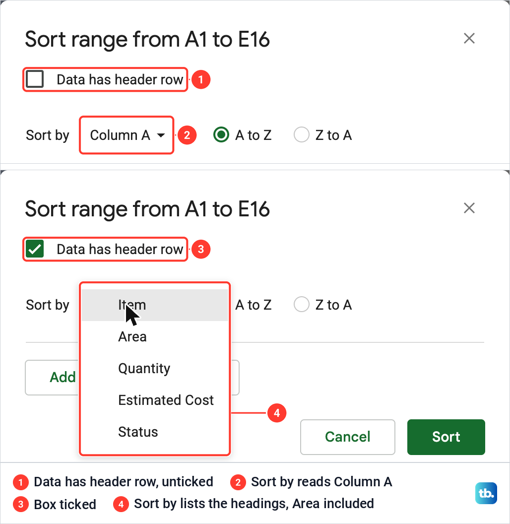
A new name only helps a sort if Sheets knows that row 1 holds headings. Select the list and choose Data > Sort range > Advanced range sorting options. Our dialog, titled Sort range from A1 to E16, opened with Data has header row unticked, although row 1 was bold and frozen, and Sort by read Column A.
Once we ticked the box, Sort by read Item, and its list offered Item, Area, Quantity, Estimated Cost and Status, with the new name Area already in it. We closed it with Cancel. Leave the box unticked and the headings are sorted in with the data, so tick it yourself.
The rest of the dialog is in our guide to sorting and alphabetizing in Google Sheets. The same Data has header row box appears when you remove duplicates in Google Sheets, and that guide found it off as well when the tool opened.
Rename a column in a table
In a table, a column's name does more than label it, because formulas can use it. We duplicated the Purchases tab from its tab menu and converted the copy, named Purchases Table. Select the list with its heading row, then choose Format > Convert to table, or press Command + Option + T on a Mac, Ctrl + Alt + T on Windows or Shift + Alt + T on ChromeOS.
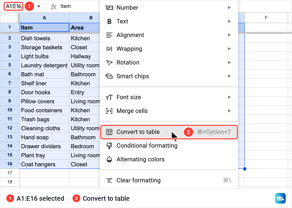
Sheets made a table named Table1, with a menu arrow beside each heading. The arrow beside the table's name opens Rename table, Adjust table range, Table header color, Table formatting, Revert to unformatted data and Delete table. We chose Rename table, typed HomePurchases and pressed Enter.
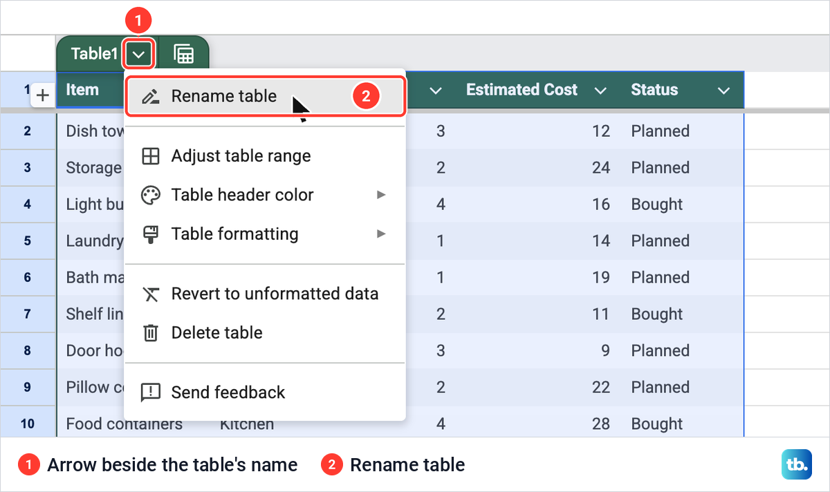
The rest of that menu is in our guide to making a table in Google Sheets. In H2, beside the table, we typed =SUM(HomePurchases[Estimated Cost]), the table's name with the heading in square brackets. It returned 225, the total of the fifteen costs.
Then we renamed the heading in D1 from Estimated Cost to Cost, by double-clicking it and typing, exactly as in a plain sheet. The formula in H2 rewrote itself to =SUM(HomePurchases[Cost]) and still returned 225, with nothing to retype.
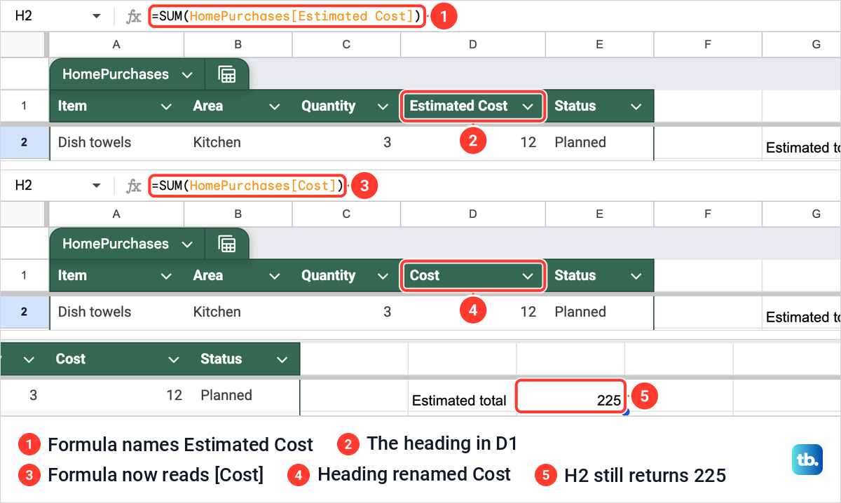
We set the heading back to Estimated Cost afterwards. A formula with plain cell addresses, such as =SUM(D2:D16), never mentions the heading, so a rename cannot affect it.
Give a range a name for formulas
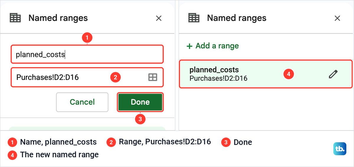
Without a table, a named range lets a formula use a name instead of D2:D16. Select the cells, D2 to D16 for our costs, then choose Data > Named ranges. A panel opens on the right with a name box, which offered NamedRange1, and the range, Purchases!D2:D16.
We typed planned_costs and clicked Done, and the panel then listed planned_costs with its range under Add a range. A range name can hold letters, numbers and underscores but no spaces or punctuation, and it cannot start with a number or look like a cell address such as A1. That is why ours has an underscore.
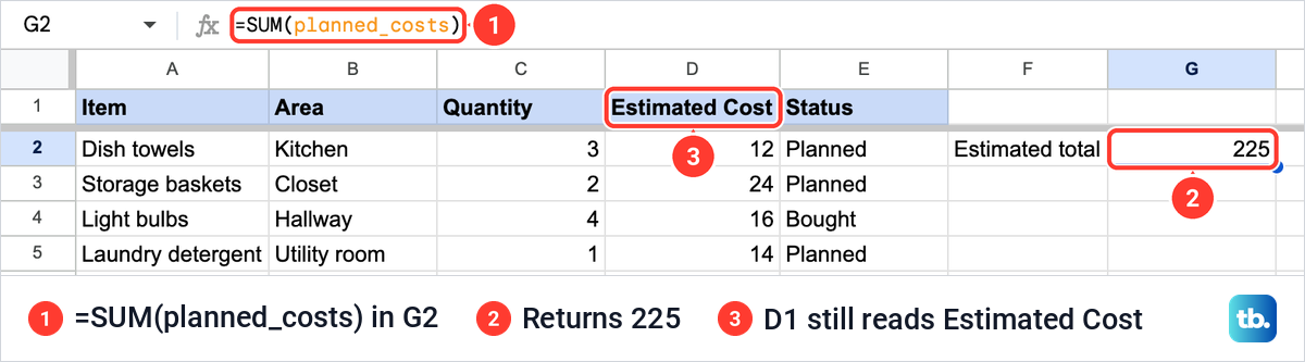
In G2 we typed =SUM(planned_costs), with the label Estimated total in F2, and it returned 225. The heading in D1 still read Estimated Cost. A named range and a visible heading are separate things, so naming the range left the heading exactly as it was.
Other things in Sheets called Rename
Two Rename entries do exist, and both are easy to mistake for a column rename. Right-click the tab at the bottom of the sheet, and its menu includes Duplicate, Copy to, Rename, Change color and Protect sheet. That Rename changes the tab's name, Purchases in our sheet, and leaves every column alone.
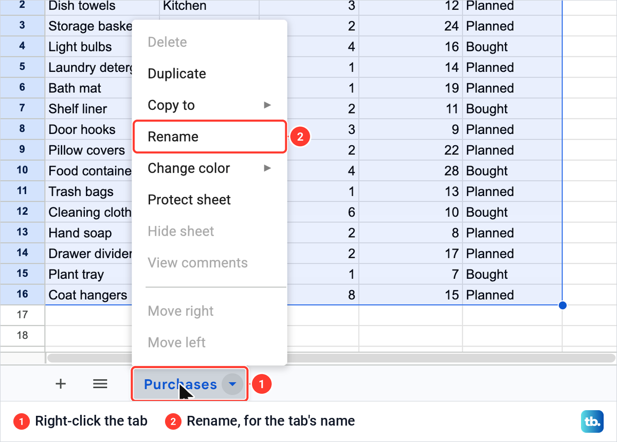
Double-clicking the text on the tab also lets you type a new name. The File menu has a Rename entry too, and that one renames the whole spreadsheet. A command called Rename column with alias belongs to Connected Sheets, which links a sheet to BigQuery data, and an ordinary spreadsheet does not have it.
Repeat the heading row on every printed page
A frozen heading row is also the row Sheets can repeat at the top of each printed page. Choose File > Print and open Headers & footers in Print settings. Under Row & column headers, a note reads "Go to View > Freeze to select which rows/columns to repeat on all pages".
On our sheet, with row 1 frozen, Repeat frozen rows was already ticked, and Repeat frozen columns was grey. Our list fitted on one page, and we left with Cancel. On a longer list, that setting puts the heading row at the top of every page.
When a heading will not change
First check where you clicked. The letter selects the whole column, while the cell under it in row 1 holds the name. If you cannot type in any cell, you probably have view or comment access, which cannot change a spreadsheet, so ask the file's owner for edit access.
If other cells accept typing but the heading does not, it may be protected. Data > Protect sheets and ranges lists what is protected. A protection may restrict editing to selected people or show a warning you must confirm. If you cannot change the heading, ask someone who can change the protection for access.
How to rename a column on Android
Open the spreadsheet in the Google Sheets app and double-tap the heading cell, such as B1. Type the new name, then tap Done. If the list has no heading row, select row 1, tap Insert and pick the option that puts the new row above row 1.
To keep the headings in view, touch and hold the row, then tap Freeze. The Android app can show named ranges but cannot add or edit them, so create those on a computer.
How to rename a column on iPhone or iPad
In the Google Sheets app, double-tap the heading cell, type the new name and tap Done. To add a heading row, select row 1, tap Insert and pick the option that puts the new row above row 1.
To freeze the headings, tap the row number, tap the right arrow in the menu that appears, then tap Freeze. Named ranges are not available in the app on iPhone and iPad.
How we tested this guide
We tested this in Google Sheets on the web in Chrome on a Mac, adding a heading row to a 15-row purchases list, renaming a heading, and checking a table column and a named range in formulas.
Frequently Asked Questions
Can I change the A, B, C column letters to words?
No. The letter's menu and its View more column actions list have no Rename entry, and the letters stayed even with gridlines off. Type the names into row 1 and freeze that row.
How do I rename a column when row 1 already holds data?
Right-click the row number 1 and choose Insert 1 row above. Your entries move down one row, and you can type the names into the new empty row 1.
Can a formula refer to a column by its name?
Yes, in two ways. In a table, use the table's name with the heading in brackets, such as =SUM(HomePurchases[Estimated Cost]). Without one, name the cells under Data > Named ranges and use =SUM(planned_costs).
Will renaming a column break my formulas?
It did not in our sheet. In a table, renaming Estimated Cost to Cost rewrote the formula to =SUM(HomePurchases[Cost]) by itself, and the total stayed 225. Formulas with plain cell addresses never mention the heading.
Why did my heading row get sorted into the data?
If you sorted a range without ticking Data has header row, Sheets treated row 1 as data. Undo the sort, then use Data > Sort range > Advanced range sorting options and tick the box before you pick a column. If you use Sort sheet A to Z from a column letter's menu instead, freeze row 1 first with View > Freeze > 1 row so the heading row stays at the top.
Can I rename a column in the Google Sheets app?
Yes. Double-tap the heading cell, type the new name and tap Done, on Android, iPhone or iPad. Make named ranges on a computer, because the apps cannot create them.
Why can't I type in the heading cell?
You may have view or comment access, which cannot change the file, so ask the owner for edit access. If other cells work, open Data > Protect sheets and ranges to see whether the heading is protected.