
To sort by date in Google Sheets, select the whole table with its headings, choose Data > Sort range > Advanced range sorting options, tick Data has header row and pick your date column. Choose A to Z for oldest to newest or Z to A for newest to oldest, then click Sort. Every row moves with its date, so each task keeps its own details.
We sorted a 15-task home schedule by its due dates in both directions. Two results are worth knowing first: the Data has header row box was off although the heading row was frozen, and a date stored as text would not sort with the real dates, one reason a date column comes out in the wrong order.
The short version
- Oldest first: select the table, choose Data > Sort range > Advanced range sorting options, tick Data has header row, pick the date column and choose A to Z.
- Newest first: follow the same steps and choose Z to A.
- The whole tab: with the heading row frozen, right-click the date column's letter and choose Sort sheet A to Z or Sort sheet Z to A.
- A sorted copy: =SORT(Schedule!A2:E16,2,TRUE) on another tab leaves the original order alone.
- Dates out of order: =ISNUMBER(B2) returns FALSE for a date stored as text. Select the date cell and choose Format > Number > Date.
- Undo a sort: press Command + Z on a Mac or Ctrl + Z on Windows and ChromeOS.
Ways to sort by date at a glance
The references match our schedule, with tasks in A1:E16 and due dates in column B. Change them to fit your sheet.
| What you need | How to do it | What changes |
|---|---|---|
| Oldest or newest first, rows kept whole | Select the table, then Data > Sort range > Advanced range sorting options, tick Data has header row, choose the date column and A to Z, or Z to A for newest first | The selected rows, in place |
| The whole tab in date order | Right-click the date column's letter, then Sort sheet A to Z or Sort sheet Z to A | Every row under the frozen heading row |
| Same-day tasks in a set order | Add another sort column in the dialog, such as then by Area | The order inside each date |
| A sort from a filtered table | Data > Create a filter, then Sort A to Z on the date heading's filter button | The rows under the filter, which stay sorted after Remove filter |
| A sorted copy | =SORT(Schedule!A2:E16,2,TRUE) on another tab | Nothing on the original tab |
| The phone app | Tap the column letter, tap the top of the column again, then More and SORT A-Z or SORT Z-A | Your data, sorted by that column |
| Command + Z on a Mac, Ctrl + Z on Windows | Press it straight after a sort | The previous order comes back |
Sort dates from oldest to newest
Select the whole table, headings included, not just the dates. Drag from the first heading to the last cell of the last row, or type the range, such as A1:E16, into the Name box at the left of the formula bar and press Enter. Our schedule had five headings in row 1 and 15 tasks below, in the order they were typed.
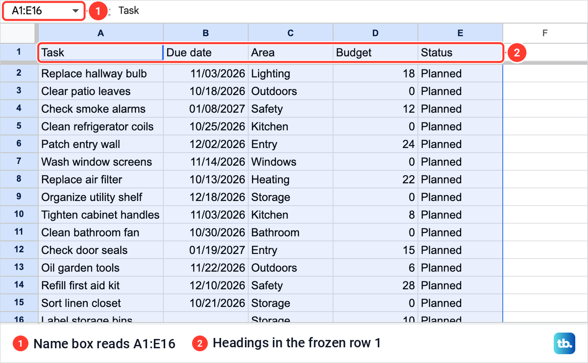
The selection is what keeps each row together, because every selected cell moves with its date. If your list has check boxes in Google Sheets for finished tasks, include that column too, so each box stays beside its task. Text columns work the same way, and our guide to alphabetizing and sorting in Google Sheets covers names and other words.
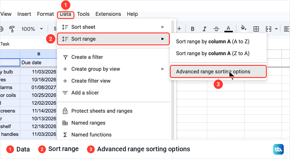
With the table selected, open Data > Sort range. On ours the submenu offered two quick sorts by column A and Advanced range sorting options, which lets you pick the date column by name.
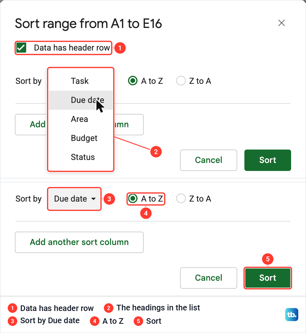
The dialog names the range, Sort range from A1 to E16 on ours. Tick Data has header row first. It was off when our dialog opened, although row 1 was frozen, and only once it was ticked did the Sort by list show our headings by name instead of Column A to Column E.
Open the Sort by list and choose your date heading, Due date on ours. Leave A to Z selected for oldest to newest and click Sort.
Our schedule now ran from 10/13/2026 to 01/19/2027, with both 2027 dates after every 2026 date. Replace air filter moved to row 2 with its Heating area, budget of 22 and Planned status, and every other task kept its own details too. The headings stayed in row 1.
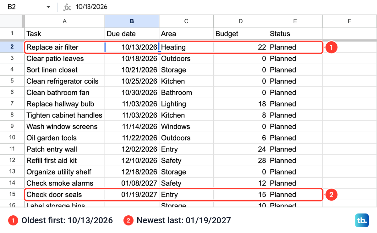
A to Z sounds like a text order, but on real dates it means oldest first, because Sheets stores each date as a count of days. Label storage bins, the one task with no due date, ended up in the last row.
Sort range is a one-time command, so a task you add later stays where you type it. Add new tasks under the table, or insert rows in Google Sheets inside it, then select the whole table again, new rows included, and sort.
Sort dates from newest to oldest
For the most recent dates at the top, repeat the same steps and choose Z to A instead of A to Z. On our schedule that put 01/19/2027 first, then 01/08/2027, then 12/18/2026 and on down to the oldest date.
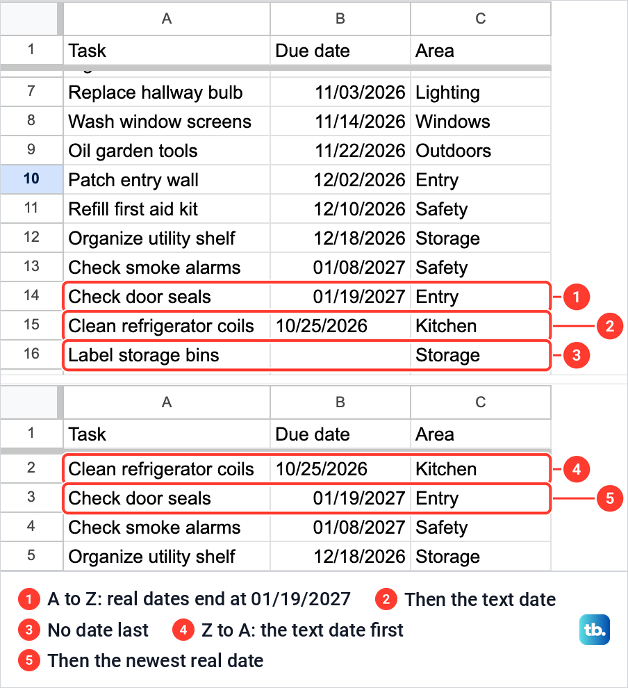
The task with no due date stayed in the last row this way too. An empty date cell went to the bottom in both directions on our sheet, so it did not push the newest dates down.
Sort the whole sheet from the column letter
Use this route when the table is alone on its tab. Right-click the letter at the top of the date column, B on ours, and choose Sort sheet A to Z for oldest first or Sort sheet Z to A for newest first.
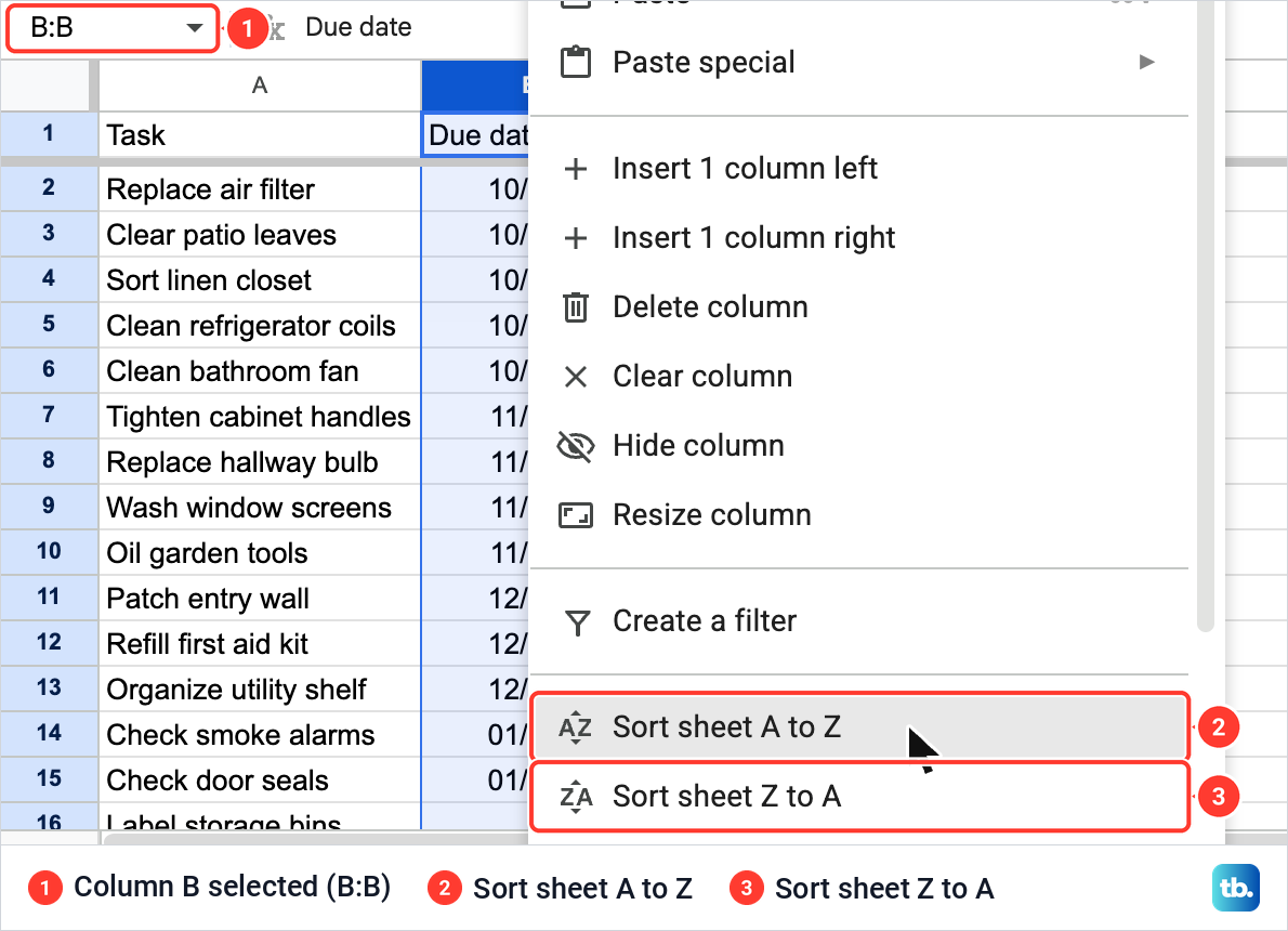
Sort sheet moved whole rows on our schedule, across every column, and left the frozen heading row where it was. That frozen row is what protects your headings here, because this route sorts the whole tab under it. If your headings are not frozen yet, freeze a row in Google Sheets before you use it.
To undo, press Command + Z on a Mac, which put our old order back, or Ctrl + Z on Windows and ChromeOS. For an older sort, click the clock icon at the top right, choose an earlier version and click Restore this version, which restores the whole file.
Break a tie when two tasks share a date
Two of our tasks were due on 11/03/2026. With the date as the only sort column, they came out as Replace hallway bulb and then Tighten cabinet handles, the order they were in before. To decide that order yourself, add a second sort column.
Select the table again and open Advanced range sorting options. Click Add another sort column, and a then by line appears with the same headings and a bin to remove it. We kept Due date with A to Z on the first line, chose Area with A to Z on the second and clicked Sort.
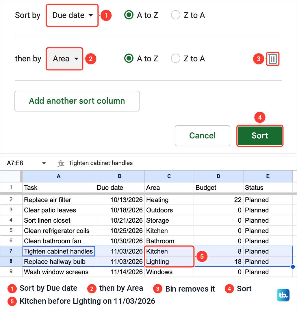
The dates still ran from oldest to newest, but the two tasks due 11/03/2026 swapped places. Tighten cabinet handles, in Kitchen, now comes before Replace hallway bulb, in Lighting, because the second column only orders tasks that share a date.
Sort dates from the filter button
A filter puts a sort button on every heading. Select the table with its headings, A1:E16 on ours, and choose Data > Create a filter. Click the filter button on the date heading and choose Sort A to Z or Sort Z to A at the top of its menu, above the filter choices.
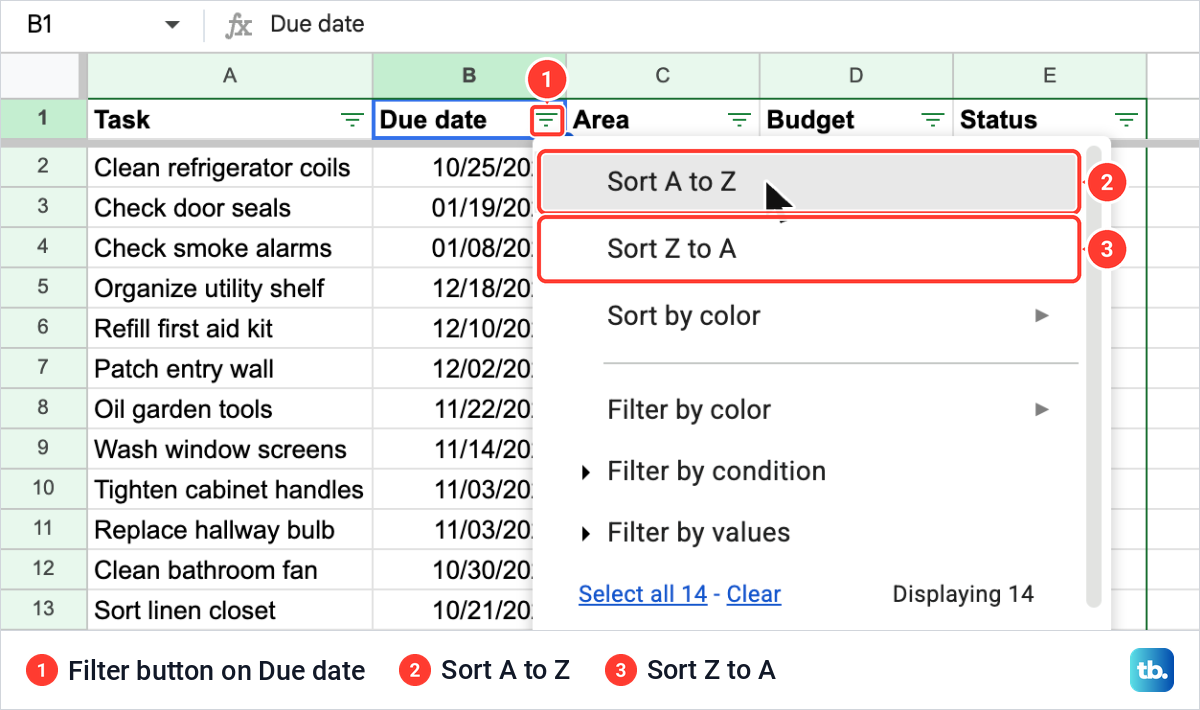
Sort A to Z gave the same oldest-first order as the dialog, with the undated task last. When we chose Data > Remove filter afterwards, the rows stayed in their new order, so you do not need to keep the filter once the dates are sorted.
A filter is part of the sheet, so anyone with access to the file sees it. To sort for yourself without changing what others see, choose Data > Create filter view on a computer and sort from the date heading inside the view.
Keep a sorted copy with the SORT function
The SORT function shows the table in date order somewhere else and leaves the original as it is. We added a tab named By due date, typed the same five headings in row 1, clicked A2 and entered this formula.
=SORT(Schedule!A2:E16,2,TRUE)Schedule!A2:E16 is the table without its headings, 2 is the date column's position counting from the first column of that range, and TRUE means oldest first. Change TRUE to FALSE for newest first.
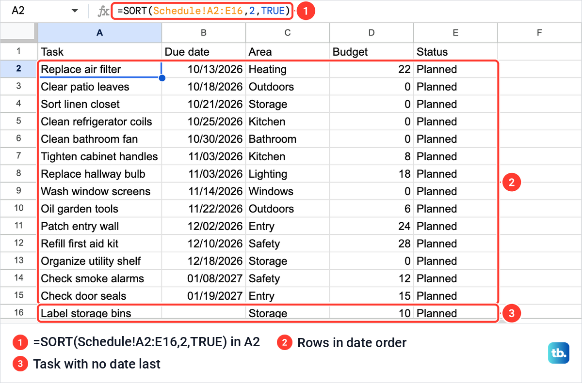
The one formula in A2 filled 15 rows, oldest date first, with the undated task last, while the Schedule tab kept its own order. The copy is formula output, so edit tasks on the original tab rather than in the copy.
Our range ends at row 16, so a task added in row 17 stays out of the copy until you extend the range in the formula. A copy in date order is also a tidy place to make a graph in Google Sheets of the budget by due date, or to total a column in Google Sheets, such as Budget.
Why some dates sort in the wrong order
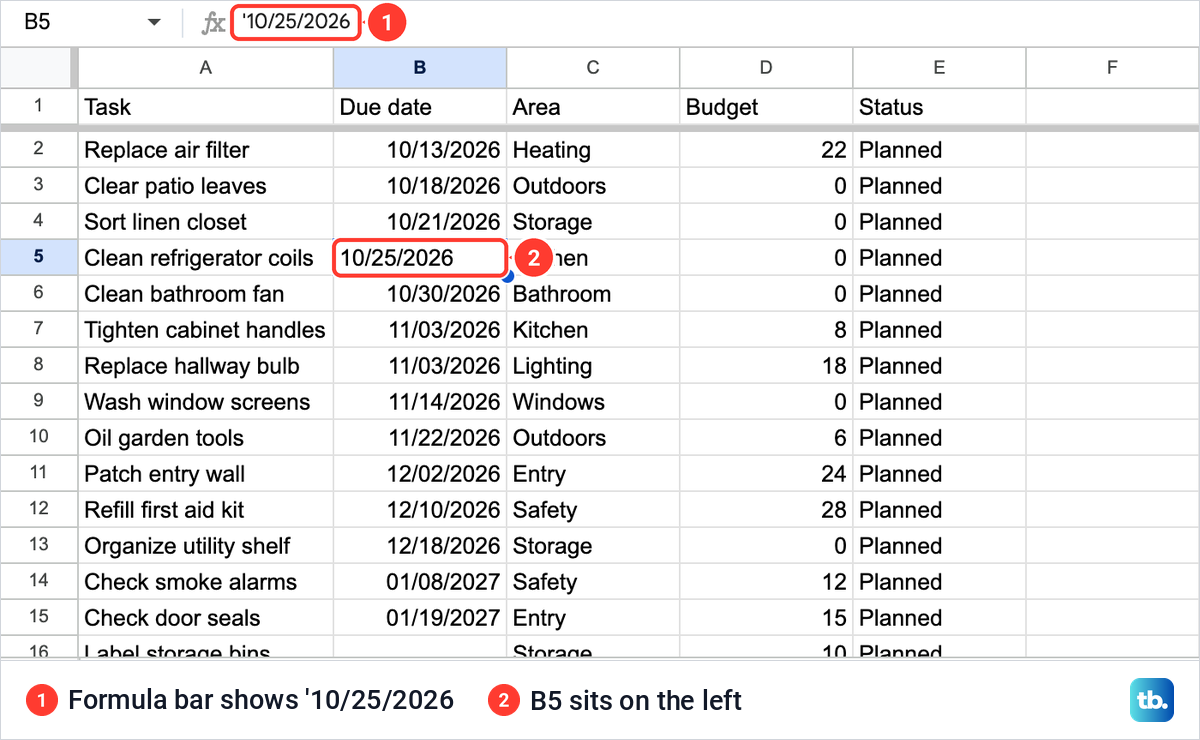
If a date column comes out in a strange order, some of its cells may hold text that only looks like a date. That can happen with dates pasted or imported from another file, and with any date typed after an apostrophe. To see it, we retyped one due date as '10/25/2026, apostrophe first.
The cell showed 10/25/2026 like the others, but on the left side of the cell, while every real date sat on the right. The formula bar still showed the apostrophe. Left alignment is the quick tell, as long as nobody has changed the column's alignment by hand.
That one cell did not sort with the rest. With A to Z it came after every real date, below 01/19/2027, even though an October 2026 date belongs near the top. With Z to A it jumped to the very first row, above the newest date, and the task with no date stayed last both ways.
A surer test than alignment is ISNUMBER, because Sheets stores a real date as a number. After the Z to A sort the text date sat in B2, so in empty cells beside the table we entered =ISNUMBER(B2) for it and =ISNUMBER(B3) for a real one. The first returned FALSE and the second TRUE.
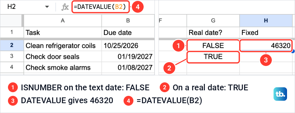
To check a whole column, put =ISNUMBER(B2) beside the first row, fill it down and look for FALSE. If there is no empty column beside the table, add a column in Google Sheets first. A FALSE next to an empty date cell is expected, because an empty cell is not a number either.
Turn text dates into real dates
Try the quickest fix first. Select the text date, or the whole date column, and choose Format > Number > Date.
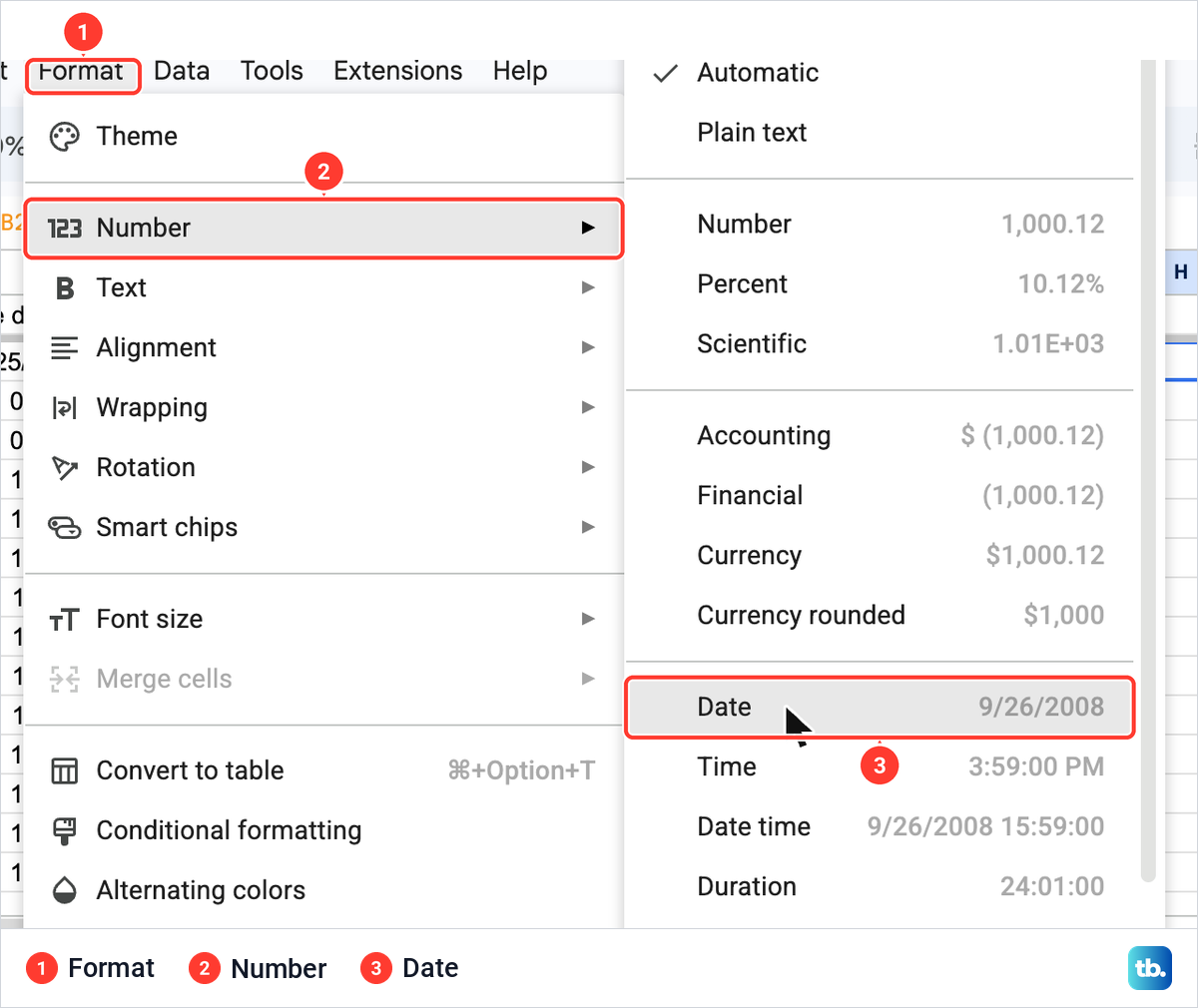
Our '10/25/2026 became a real date straight away. It moved to the right of its cell, the apostrophe disappeared from the formula bar and ISNUMBER changed to TRUE. The next sort put it between 10/21/2026 and 10/30/2026, where it belongs.
If a cell does not change, try DATEVALUE in an empty cell beside it. We entered =DATEVALUE(B2) for the text date and got 46320, the same date as a count of days, which read 10/25/2026 once formatted with Format > Number > Date. That result means Sheets can read the date, so retype it in the original cell without the apostrophe and sort the table again.
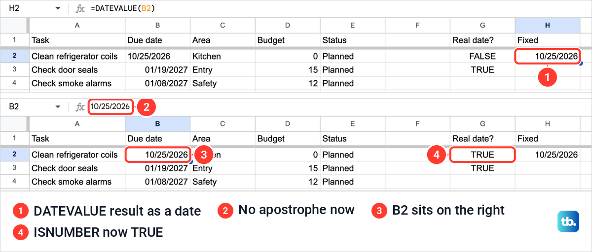
DATEVALUE does not tell you whether a date is real, though. On a real date in our sheet it returned a number as well, with no error, so use ISNUMBER to tell text from a real date.
Dates written in an order Sheets does not expect may not convert at all. Sheets reads dates by the spreadsheet's locale under File > Settings, and changing it changes the date, number and currency formats for everyone using the file, so check it before you retype a column of day-first dates.
Sort by date in the Google Sheets app
On an Android phone or tablet, open the spreadsheet, tap the letter above the date column, then tap the top of the column again to open the menu. Tap More, scroll down and tap SORT A-Z or SORT Z-A.
On an iPhone or iPad the steps are the same, ending with More and SORT A-Z or SORT Z-A. Filter views are not in the phone apps, so set up a personal sort order on a computer.
How we tested this guide
We tested this in Google Sheets on the web in Chrome on a Mac, sorting a 15-task schedule by its due dates in both directions, with one date missing and one stored as text.
Frequently Asked Questions
How do I sort dates from newest to oldest in Google Sheets?
Select the whole table, choose Data > Sort range > Advanced range sorting options, tick Data has header row, pick the date column and choose Z to A. For a table alone on its tab, freeze the heading row, then right-click the date column's letter and choose Sort sheet Z to A.
Why are my dates not sorting correctly in Google Sheets?
Some cells may hold text that looks like a date, which sits on the left of the cell and sorts apart from the real dates. Check with =ISNUMBER(B2), which returns FALSE for text, then select those cells and choose Format > Number > Date.
How do I keep rows together when sorting by date?
Select every column of the table before you sort, not only the dates. Sort sheet from the column letter also moved whole rows on our sheet and left the frozen heading row in place.
Can Google Sheets sort by date automatically?
A SORT formula on another tab, such as =SORT(Schedule!A2:E16,2,TRUE), shows the list in date order without changing the original. On our sheet one formula filled all 15 rows in date order. Tasks added below row 16 need the range in the formula extended.
Where do blank dates go when I sort?
On our sheet, the task with an empty date cell went to the last row with both A to Z and Z to A. A date stored as text behaved differently, sorting after every real date with A to Z and before them all with Z to A.
How do I sort by date on Android or iPhone?
Open the sheet in the Google Sheets app, tap the date column's letter and tap the top of the column again. Tap More, then SORT A-Z or SORT Z-A.