


To alphabetize in Excel, click one cell in the column you want in order, such as any name in a Name column, then select Data > Sort A to Z. In a list with no blank rows or columns, Excel sorts it by that column and moves each row with it. For reverse order, use Sort Z to A.
On our list the header row stayed on top, and if yours moves, the header fix below covers the setting to check. Select only the names instead and Excel asks whether to bring the neighbouring columns along, so leave Expand the selection chosen and the rows stay whole. If you want a sorted copy and the original left alone, the SORT function does that in a few keystrokes.
Two settings catch people out. Clearing My data has headers dropped our header row into the middle of the list, and Excel for the web's Sort On menu opened with four choices even though Microsoft's help says it is switched off.
The short version
- A to Z: click one cell in the column, then Data > Sort A to Z, or press Alt, A, S, A one after another.
- Keep rows together: if a Sort Warning appears, leave Expand the selection chosen and select Sort.
- Two columns: select Data > Sort, pick the first column, then Add Level for the second.
- A sorted copy: type
=SORT(A2:C5,2,1)in an empty cell beside the list, using your own range and the number of the name column. - Changed your mind: press Ctrl + Z straight after the sort.
Ways to alphabetize in Excel at a glance
| Method | What it does | Do the original rows move? | Best for |
|---|---|---|---|
| Data > Sort A to Z or Alt, A, S, A | Sorts the list A to Z by the column you clicked | Yes, whole rows move together | A quick one-off sort |
| Data > Sort Z to A or Alt, A, S, D | Sorts the list Z to A | Yes, whole rows move together | Reverse order |
| Data > Sort with Add Level | Sorts by one column, then another, such as Team then Name | Yes | Grouped lists |
| Table header arrow, after Ctrl + T | Sorts a table from the arrow on its header | Yes | A list you sort often |
=SORT or =SORTBY | Shows a sorted copy in empty cells, in Microsoft 365 and Excel 2021 or later | No, the source stays as it is | Reports and lists that must keep their order |
| Excel for the web, Data > Sort Ascending | The same sorts in a browser, with labelled buttons | Yes | Files in OneDrive or SharePoint |
Every method except the formulas rearranges the cells themselves, so make a copy of the Excel file first if the original order matters to you. Ctrl + Z straight after a sort also brings the old order back, as the table section shows.
Sort a column from A to Z or Z to A
Click one cell in the column you want to alphabetize, such as B2 under a Name heading. You do not need to select the column or the list. Open the Data tab and select the small A over Z button at the top left of the Sort & Filter group. If a green tip about importing data covers the sheet the first time you open the tab, select Got it.
Its ScreenTip reads Sort A to Z, with Lowest to highest underneath, even when the column holds text. On our sheet, with only B2 selected, one click turned Zoe, Amy, Ben, Eli into Amy, Ben, Eli, Zoe. The IDs moved with their names (102 Amy, 103 Ben, 104 Eli, 101 Zoe), the Team column came along, and the header stayed in row 1 with no warning.
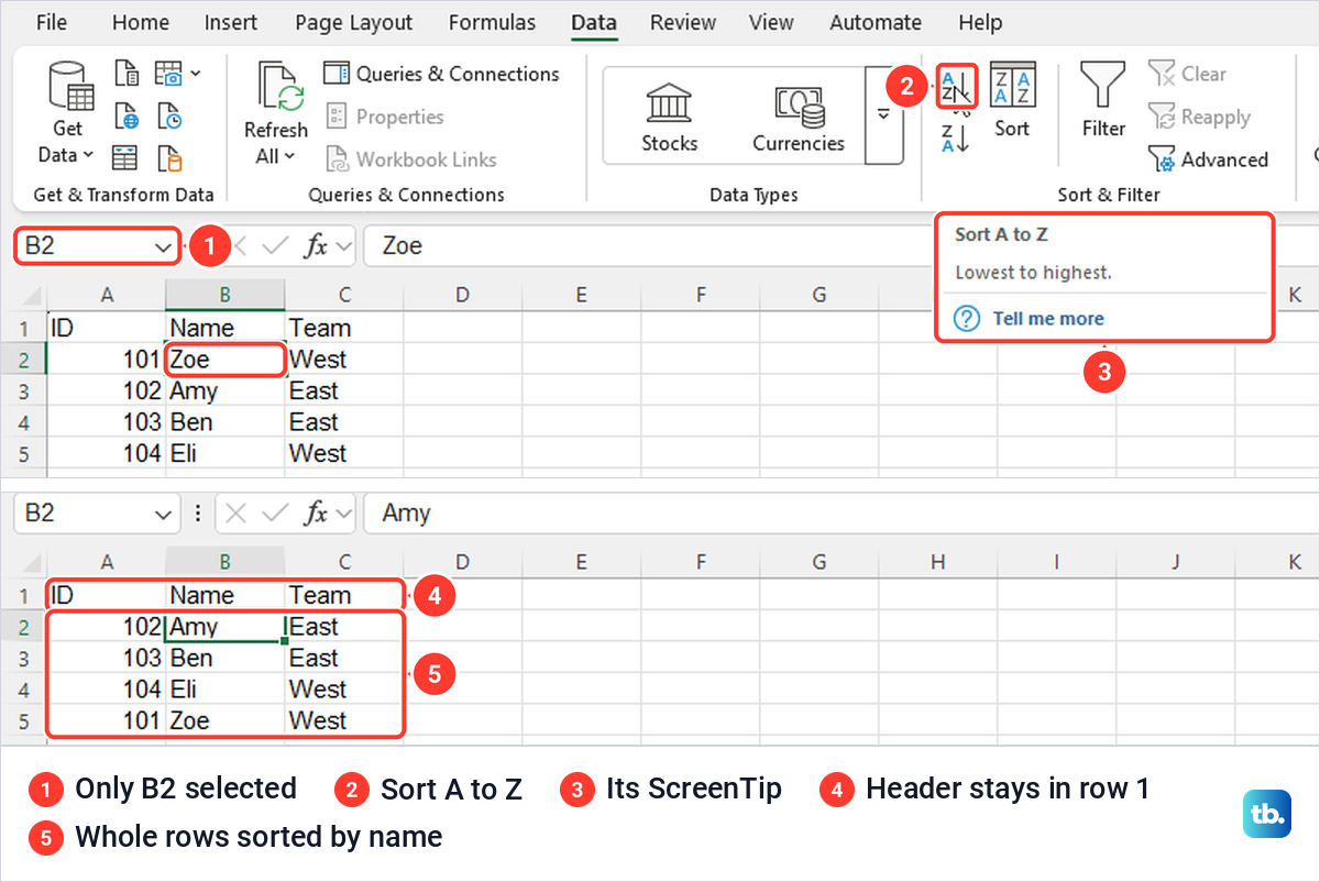
For reverse order, use the button underneath, Sort Z to A. Sorting also puts repeated names side by side, which makes them easy to spot before you remove duplicates in Excel.
The same two commands sit on the Home tab under Sort & Filter, above Custom Sort and Filter. From there, Sort Z to A put Zoe first and Amy last on our sheet, again moving whole rows.
Use the keyboard instead
Ribbon key tips turn the sort into four keys. Press Alt, then A for the Data tab, then S, then A, one key after another rather than together. After S, our screen showed only three tips, SA for Sort A to Z, SD for Sort Z to A and SS for the Sort dialog, and the full sequence sorted our list A to Z.
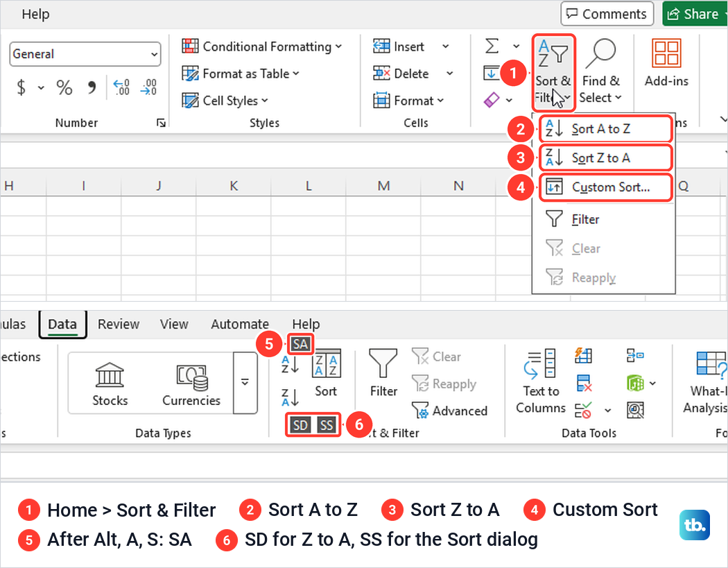
Alt, A, S, S opens the full Sort dialog used in the two-column section below. Both sequences sit well with the other Excel keyboard shortcuts worth learning if you sort lists often.
Keep the rest of each row with the name
Alphabetizing goes wrong when the names move and the rest of the row does not. When we selected only the names, B2:B5, and chose Sort A to Z, a Sort Warning box said Excel had found data next to the selection and would not sort it, because it was not selected.
The box offered Expand the selection, already chosen, and Continue with the current selection. Leave the first one and select Sort. On our sheet that sorted the IDs and teams along with the names, exactly as the one-cell method did.
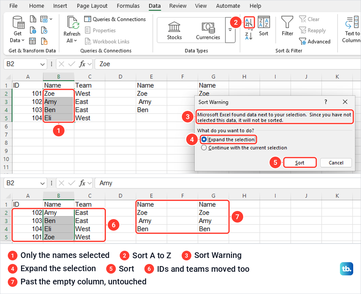
Continue with the current selection sorts the selected names on their own. Microsoft's example shows what follows: employees end up associated with different departments than they were before. If you pick it by mistake, press Ctrl + Z straight away.
Excel works out where a list ends from empty rows and columns. On our sheet, Expand the selection took in columns A to C and stopped at the empty column D, so the separate lists in columns E and G stayed as they were. Microsoft's layout advice matches that: at least one blank column and one blank row between separate lists, and no blank rows or columns inside one.
Hidden rows are another trap. Microsoft says hidden rows are not moved when you sort rows, so they stay where they are and miss the sort. Unhide them before a big sort with Unhide Rows, which sits on the same menu as the column commands in our guide to unhide hidden columns in Excel.
Sort by two or more columns
To group a list and alphabetize inside each group, such as team first and then name, use the Sort dialog. Click a cell in the list and select the large Sort button on the Data tab. Check that My data has headers is ticked, so the columns are listed by their header names.
On a sheet we had never sorted, the Sort by box opened empty, with Sort On set to Cell Values and Order set to A to Z. On a sheet we had sorted before, it opened with the last sort, Name and A to Z, already filled in. Always check that box rather than trusting what is there.
Choose Team in Sort by. Select Add Level, which adds a Then by row, and choose Name in it. Leave both orders on A to Z and select OK.
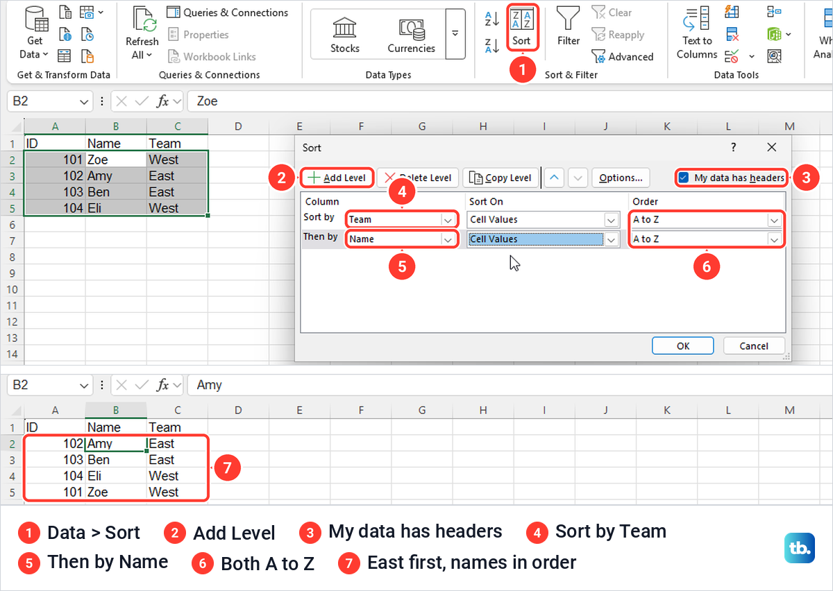
Our list came out as Amy and Ben in East, then Eli and Zoe in West, every row whole. Excel sorts by the first level and only uses the second to order rows that tie on the first, so the East names come before the West names and each team is alphabetized inside.
The Order list offers A to Z, Z to A and Custom List, which is for orders such as weekdays rather than the alphabet. Sort On can also sort by Cell Color, Font Color or Conditional Formatting Icon instead of the text itself.
Sort an Excel table from its header
If you sort the same list often, turn it into a table. Click a cell in the list and press Ctrl + T. Our Create Table box showed the range =$A$1:$C$5 and a ticked My table has headers box, and OK added an arrow to each header.
Pressing Ctrl + T only creates the table; it does not sort anything. Select the arrow on the Name header and choose Sort A to Z. Our table sorted to Amy, Ben, Eli, Zoe with every ID still beside its name and the header on top, and the Name arrow then showed a small sort icon so you can see which column the table is sorted by.
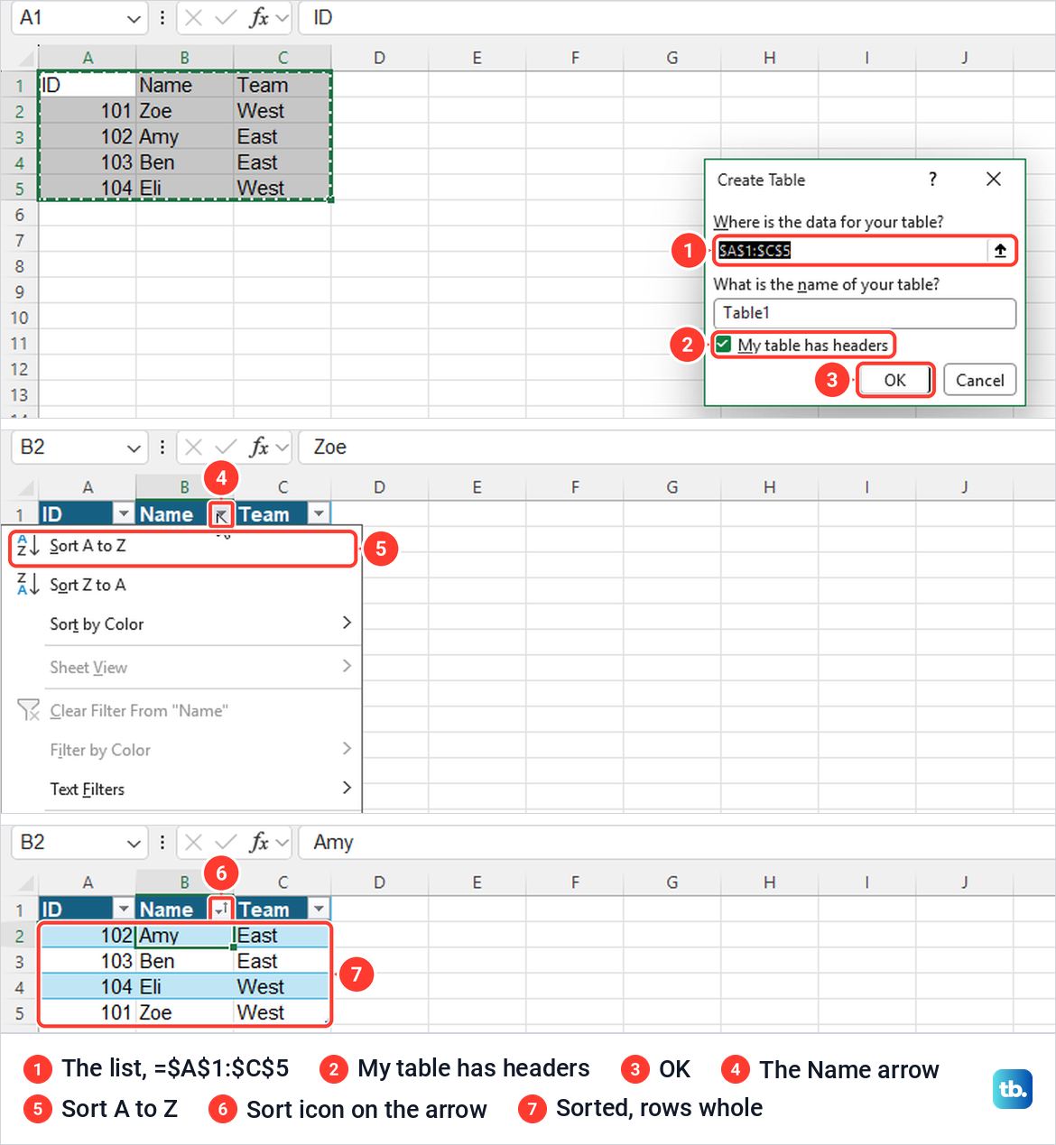
We pressed Ctrl + Z straight after the sort and the original order came back, and Ctrl + Y sorted it again. Undo is also Microsoft's answer for any sort that goes wrong, so check the result before you carry on editing.
If the header arrows are missing or do nothing, fix filters that are not working in Excel before you sort. On a long list it also helps to freeze the header row in Excel, so the column names stay in view while you check the new order.
Make a separate sorted copy with a formula
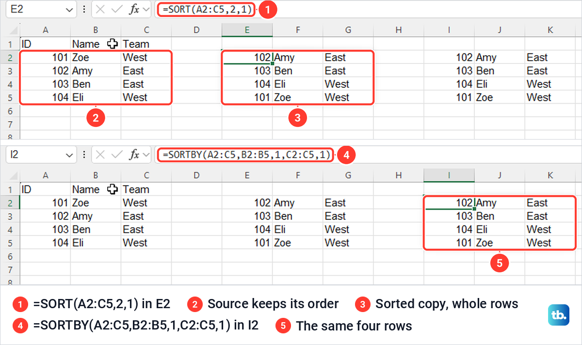
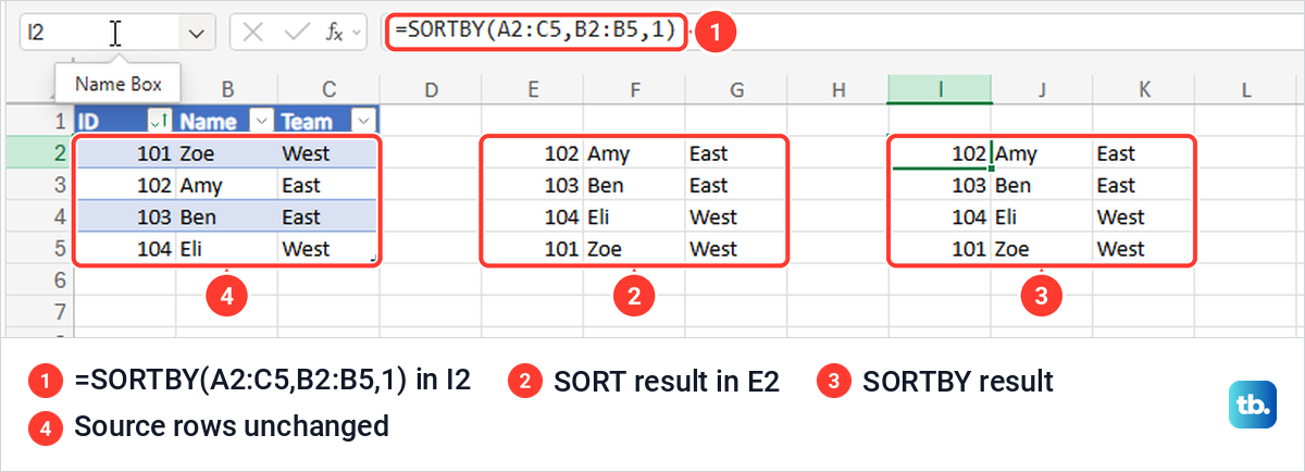
The SORT function leaves your list where it is and shows an alphabetized copy somewhere else. With our list in A1:C5, we clicked E2, typed =SORT(A2:C5,2,1) and pressed Enter. Excel spilled four complete rows into E2:G5 in name order, inside a thin blue border, and the original A2:C5 still read Zoe, Amy, Ben, Eli.
The three parts are the rows to sort, without the header, the column of that range to sort by, 2 for Name, and the order. Microsoft lists 1 for ascending order, which is also the default, and -1 for descending, so change the last 1 to -1 for Z to A.
SORTBY sorts by a range you name instead of a column number, which reads more clearly with several keys. In I2 we typed =SORTBY(A2:C5,B2:B5,1,C2:C5,1), which sorts by name and then by team, and it returned the same four rows. Microsoft notes that each range you sort by must be one column wide and cover the same rows as the list.
Microsoft lists SORT and SORTBY for Excel for Microsoft 365, Excel 2024 and Excel 2021, on Windows and Mac, and both also worked in Excel for the web on our test. In an older version without them, sort a copy of the list with Data > Sort A to Z instead.
A fixed range such as A2:C5 does not take in names you add in row 6. Microsoft says a SORT formula based on an Excel table resizes as rows are added or removed, as long as it uses the table's structured references. Keep the cells the result needs empty, or the formula shows #SPILL! instead of the list.
Alphabetize in Excel for the web
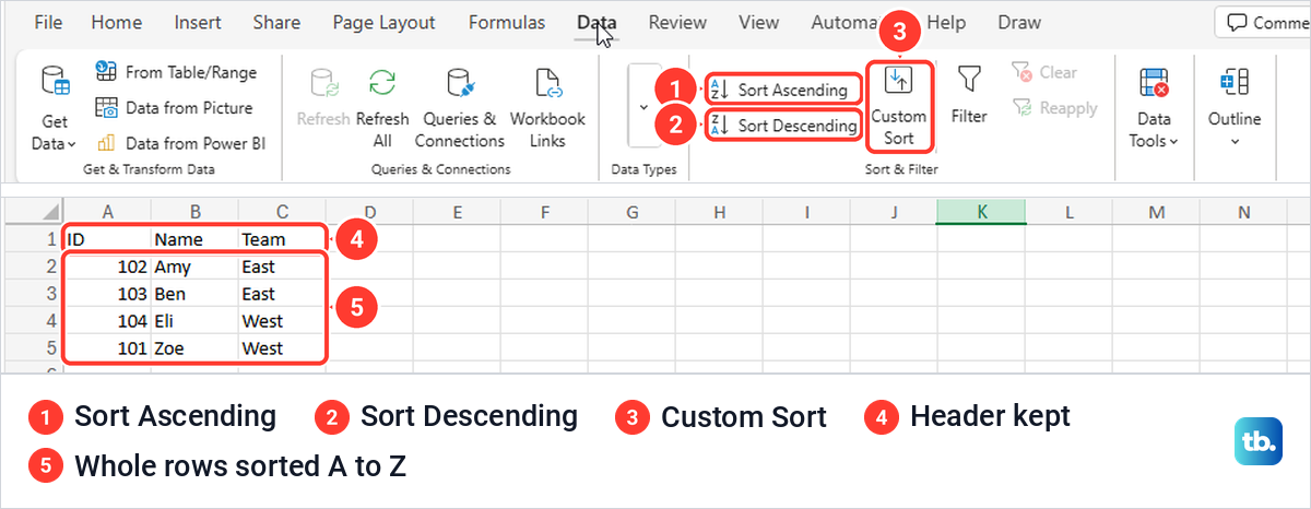
Excel for the web sorts the same way, with clearer button names. Click a cell in the column, open the Data tab and select Sort Ascending for A to Z or Sort Descending for Z to A. Both are labelled buttons in the Sort & Filter group, beside Custom Sort.
In Microsoft Edge, with B2 selected, Sort Ascending gave us Amy 102, Ben 103, Eli 104 and Zoe 101, and Sort Descending reversed it. Whole rows moved and the header stayed on top, as on the desktop. If you have not used Excel in a browser before, our Excel for beginners guide shows where to find it.
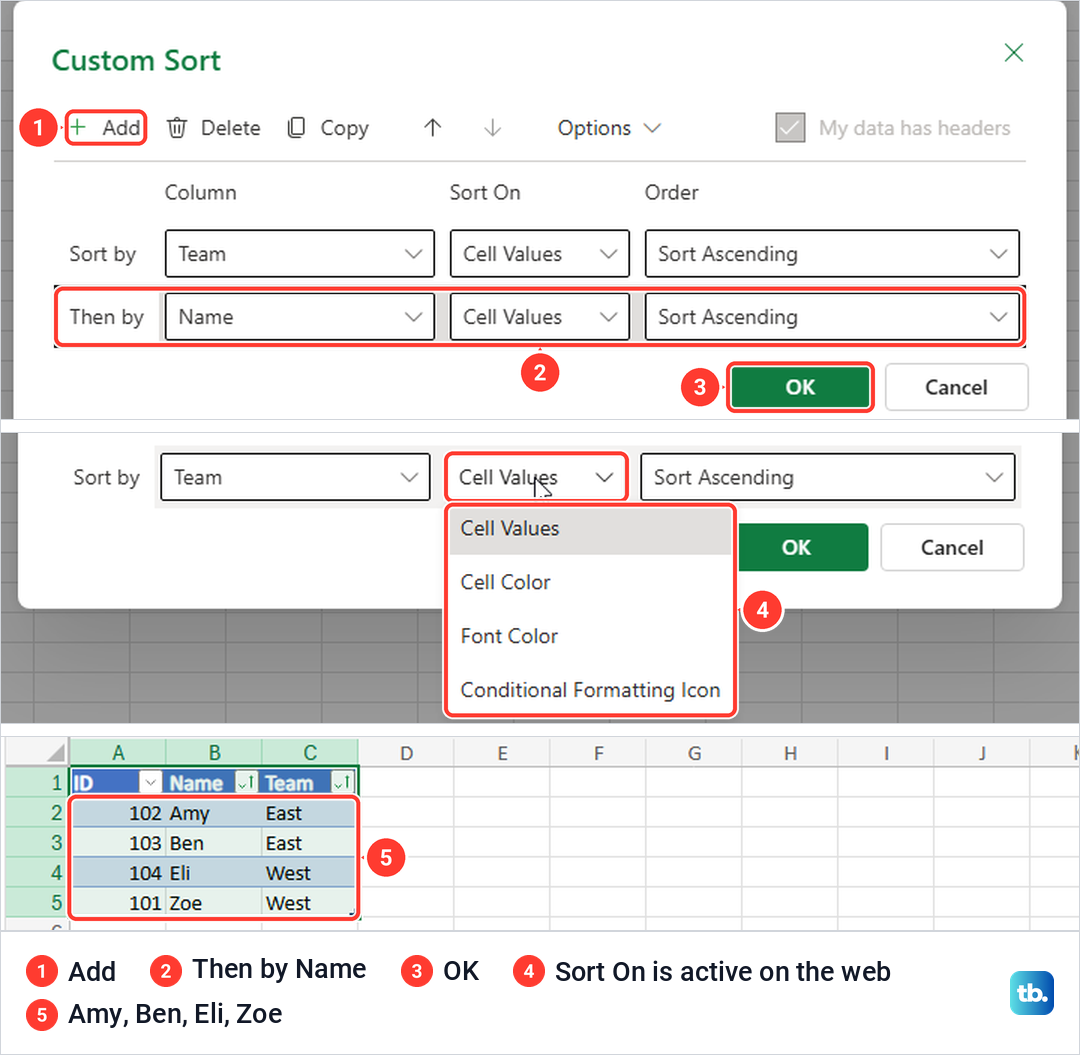
For two keys, select Data > Custom Sort. The web dialog says Add where the desktop says Add Level, and its Order list offers only Sort Ascending and Sort Descending, with no Custom List. We sorted by Team, added Name as the Then by row and selected OK, and a list we had put in Z to A order came out Amy, Ben, Eli, Zoe.
Microsoft's help page says the web Sort On menu is disabled because it is not yet supported. In our browser it was active and listed Cell Values, Cell Color, Font Color and Conditional Formatting Icon, the same four choices as the desktop app. The dialog also opened filled in with the table's current sort, so check each row before you select OK.
Header arrows work on a web table too, and the Name arrow's menu adds Custom Sort and an active Sheet View entry to the desktop list. =SORT(A2:C5,2,1) and =SORTBY(A2:C5,B2:B5,1) each spilled Amy, Ben, Eli and Zoe in the browser and left the source rows untouched.
Fix a header that sorts into the list
If your column names end up in the middle of the list, Excel treated the header row as data. The setting is My data has headers, in the dialog you open with Home > Sort & Filter > Custom Sort or Data > Sort. When we cleared it, the column list changed from the header names to Column A, Column B and Column C, and row 1 was highlighted with the data.
Sorting Column B from A to Z then dropped the ID, Name, Team row into row 4, between Eli and Zoe, because Excel alphabetized the word Name along with the names. Ctrl + Z put it back. With the box ticked again and Sort by set to Name, the header stayed in row 1 and every ID stayed with its name.
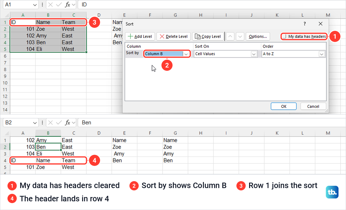
Microsoft's rule is simple: tick My data has headers when the first row of the range you are sorting holds headings, and clear it when that row holds data. Remember that a sort is a one-time change, so names typed under the list later stay at the bottom. When you insert a new row in Excel for another record, sort the list again afterwards.
Fix sorting on a protected sheet
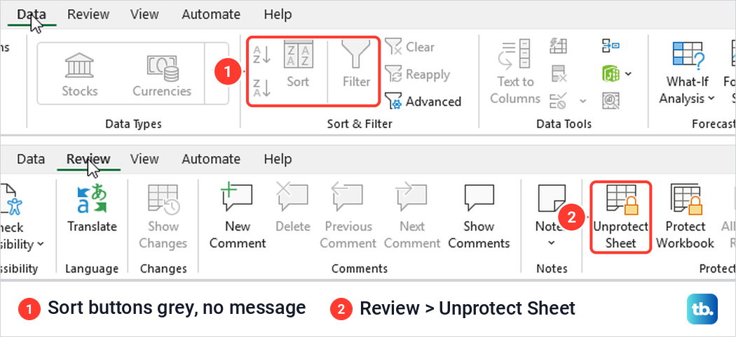
If the sort buttons are grey and clicking them does nothing, one cause is a protected sheet. On our protected sheet, Sort A to Z, Sort Z to A, Sort and Filter were all greyed out on the Data tab, and a click produced no message at all. Check the Review tab: if it shows Unprotect Sheet instead of Protect Sheet, protection is on.
The Protect Sheet box has a Sort option, but ticking it did not help on our sheet. With Sort allowed and the cells still locked, Sort A to Z still would not run.
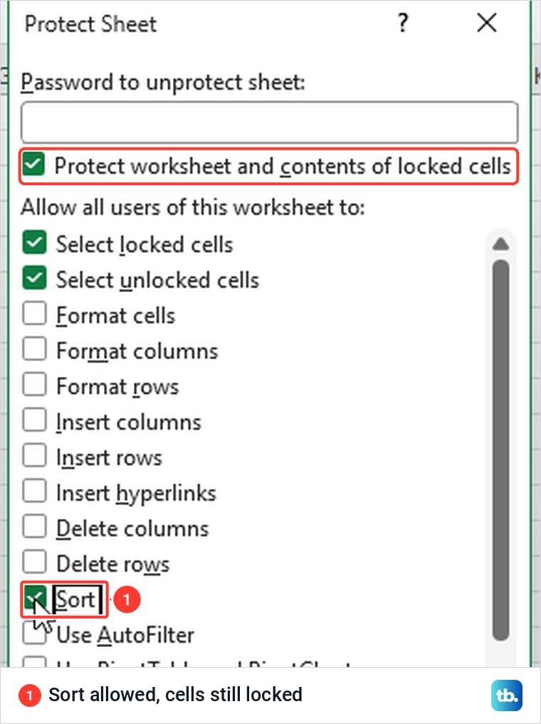
Instead, Excel showed the message "The cell or chart you're trying to change is on a protected sheet" and told us to unprotect the sheet. Microsoft explains why: users can't sort ranges that contain locked cells on a protected worksheet, regardless of that setting.
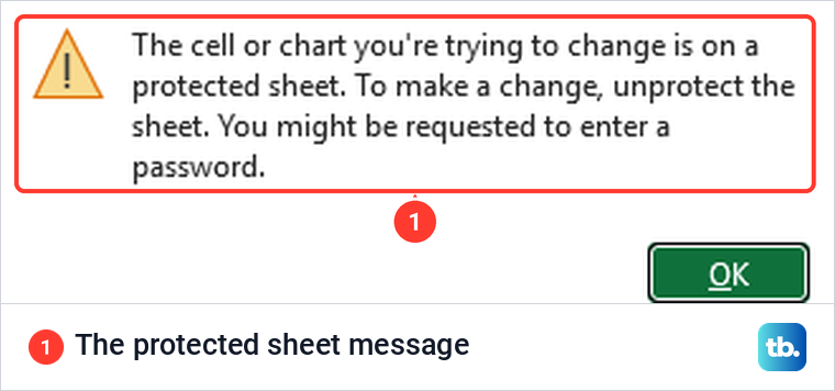
Select Review > Unprotect Sheet and type the password if Excel asks for it, and our list sorted normally straight after. If you do not know the password, ask whoever protected the sheet, and see our guide to unprotect an Excel worksheet . To let others sort a protected sheet, clear the Locked box for the cells they sort, as our guide to lock cells in Excel explains, then tick Sort in the Protect Sheet box.
Fix the merged cells error
Merged cells of different sizes can stop a sort. We merged G2:G3 in a short list with Home > Merge & Center, and Excel first warned that merging cells only keeps the upper-left value and discards other values. Sorting the list then failed with the message "To do this, all the merged cells need to be the same size."
Microsoft's help article quotes the message as "This operation requires the merged cells to be identically sized", but the fix is the same. Select the merged cell, open the arrow beside Merge & Center and choose Unmerge Cells, then sort again. Our guide on how to unmerge cells in Excel has more ways to do it.
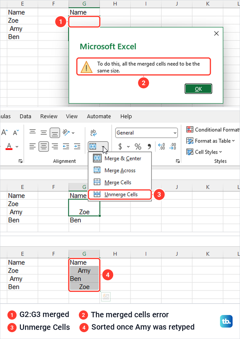
Unmerging does not bring back what the merge threw away. Amy, the name in the lower cell, was gone after we unmerged, and we had to type it again before the list sorted to Amy, Ben, Zoe. The centred alignment from Merge & Center also stayed on the cells and moved with the names.
Fix names that sort in the wrong place
A space before a name is easy to miss in the cell, but Excel counts it. We typed one space before Zoe, and Sort A to Z put Zoe at the top of the list, above Amy and Ben, because the space counted ahead of the letters. Click the cell and look in the formula bar, where the space shows as a gap before the first letter.
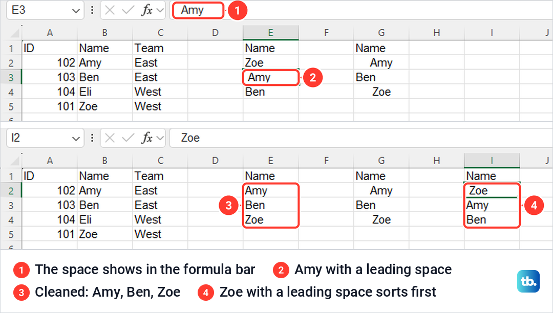
Delete the space by hand, or for a long list clean the names with the TRIM function, as Microsoft suggests. After we removed the space, the list sorted Amy, Ben, Zoe. Our guide to fix the TRIM function in Excel shows the helper column, the Paste Special > Values step that puts the cleaned names back, and what to do when a non-breaking space survives TRIM.
Fix a SORT formula that shows #SPILL!
SORT needs empty cells to spill into. We typed BLOCK in E3 and entered =SORT(A2:C5,2,1) in E2, and E2 showed #SPILL! with a dashed outline around E2:G5, the area the result needed, and a small warning button beside it.
Select the button and its menu opens with Spill range isn't blank at the top. Choose Select Obstructing Cells and Excel jumps to the cell in the way, E3 on our sheet. Delete or move what is there and the list spills straight away, as ours did once E3 was empty.
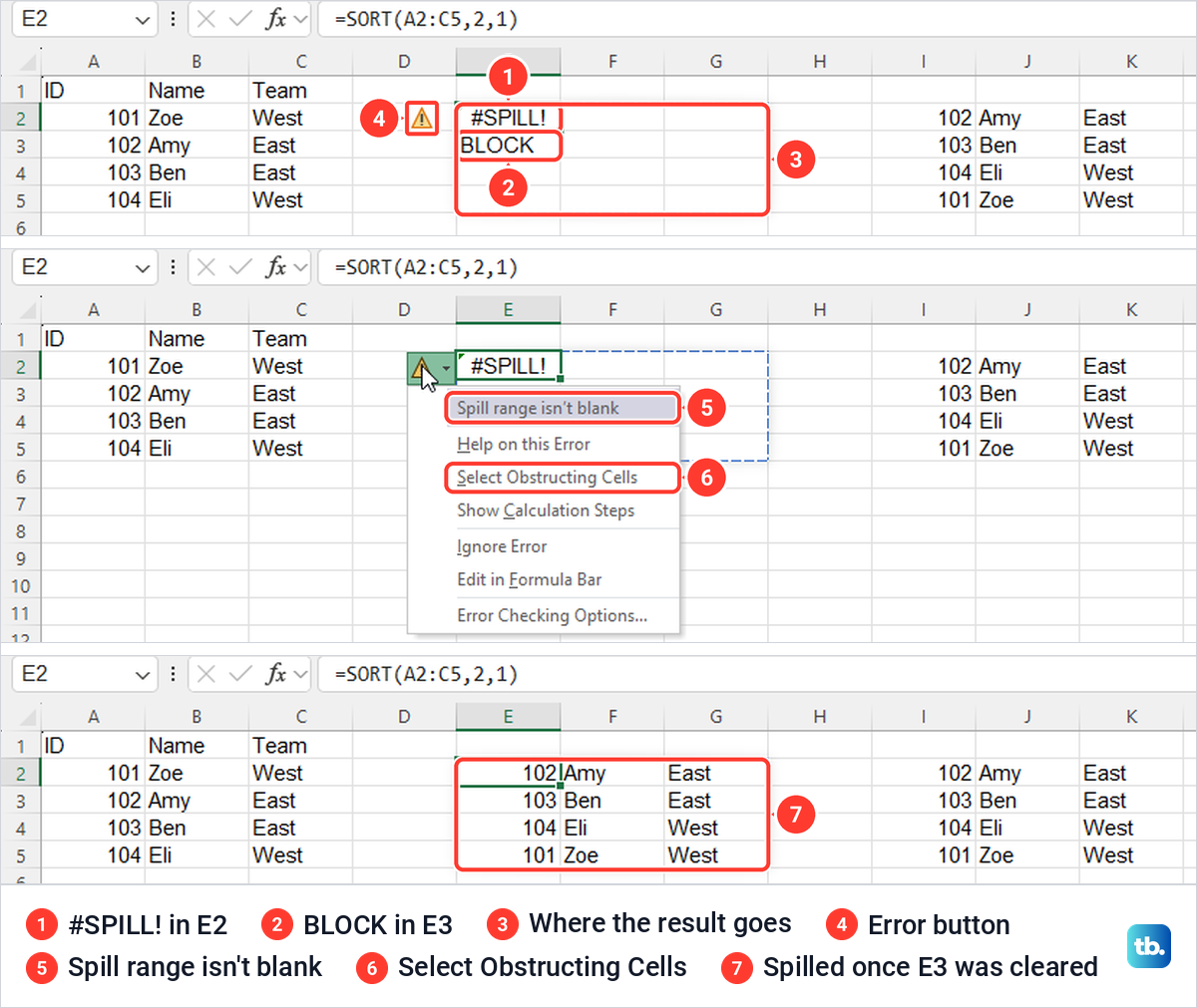
Microsoft lists merged cells inside the spill area as another cause of the same error. If SORT still shows an error once the area is clear, fix Excel formulas that are not working before you change the data.
Sort by last name, by case or on a Mac
To sort by last name when first and last names are in separate columns, use Data > Sort with Last name in Sort by and First name on an Add Level row. If full names share one cell, Excel sorts by the whole text, which starts with the first name, so put the last name in a column of its own first. Microsoft's way to split it is the Convert Text to Columns Wizard or text functions.
The Options button in the Sort dialog holds Case sensitive, and Sort left to right for data laid out across a row, which Microsoft says tables do not support until you convert them to a range. Custom List in the Order box sorts by an order you define, such as weekdays.
In Excel for Mac, Microsoft's steps are to click a cell in the column, then select Ascending or Descending on the Data tab. Data > Sort adds more levels there.
For a workbook in OneDrive or SharePoint that others are editing, Microsoft describes Sheet Views under View > Sheet View > New, and says Excel may ask whether to apply a sort for just you or for everyone. Its help page also warns that when you use Sheet View in desktop Excel and save, the sorts you made appear in the Default view for all users.
How we tested this guide
We tested this in Excel for Microsoft 365 on Windows 11, version 25H2, and Excel for the web in Microsoft Edge, sorting a made-up list of names and teams.
Frequently Asked Questions
How do I alphabetize in Excel without mixing up the rows?
Click one cell inside the list rather than selecting the column, then use Data > Sort A to Z. If a Sort Warning appears, keep Expand the selection chosen, and Excel moves each row with its name, as it did on our sheet.
How do I alphabetize a column and keep the header at the top?
Make sure My data has headers is ticked in the Sort dialog. When we cleared it, the header row sorted into the middle of our list.
Can I sort by last name and then first name?
Yes, if they are in separate columns. Select Data > Sort, choose the last name column, then select Add Level and choose the first name column.
Will the SORT function change my original list?
No. It shows a sorted copy in empty cells and leaves the source as it was, which is what =SORT(A2:C5,2,1) did on our sheet.
Why is Sort greyed out in Excel?
A protected sheet is one cause, and it greyed out the sort buttons on ours. Select Review > Unprotect Sheet, with the password if one was set, and the sort buttons work again.
Can I undo an alphabetical sort?
Yes, press Ctrl + Z straight after the sort. On our sheet it restored the original order at once, and Ctrl + Y sorted the list again.
How do I alphabetize in Excel for the web?
Click a cell in the column and select Data > Sort Ascending or Sort Descending. Use Data > Custom Sort to sort by two columns, such as Team and then Name.