


To split cells in Excel, select the column that holds the text, open Data > Text to Columns, choose Delimited, tick the separator your text uses, such as a comma or a space, set an empty Destination cell and select Finish. Each part lands in its own column. The same steps separate names in Excel when every name is a first and last name with one space between them.
Excel cannot cut one ordinary cell into two smaller cells the way a Word table can. Splitting a cell means moving its contents into the cells beside it or, if the cell was merged earlier, unmerging it.
The short version
- Text into columns: select one column, then Data > Text to Columns, Delimited, tick the separator, pick an empty Destination and select Finish.
- First and last names: type the first name beside the first full name, select the cell below it and press Ctrl + E, then do the same for the last name.
- Results that update: type
=TEXTSPLIT(A2,",")in an empty cell to split across, or=TEXTSPLIT(A2,,",")to split down. - A merged cell: select it, then Home > Merge & Center arrow > Unmerge Cells.
- Excel for the web: Data > Data Tools > Split Text to Columns replaced the original text on our sheet, so split a copy.
Choose the right way to split cells in Excel
The right tool depends on what is in the cell and whether the result should update later. Text to Columns types fixed values into new cells and Flash Fill fills a column from your examples, while TEXTSPLIT is a formula that follows its source. Unmerging is a different job, because it only separates cells that were joined together.
| Method | Best for | What you get | The original text |
|---|---|---|---|
| Data > Text to Columns, Delimited | Text with commas, spaces or another separator | Fixed values in new columns | Kept if the Destination is an empty cell |
| Text to Columns, Fixed width | Codes that split at the same position | Fixed values in new columns | Kept if the Destination is an empty cell |
| Flash Fill, Ctrl + E | Names and other clear patterns | Values filled in from your examples | Kept |
=TEXTSPLIT() | Results that change when the text changes | A formula that spills across or down | Kept |
=TEXTBEFORE() and =TEXTAFTER() | Only the first part, or everything after it | One formula result each | Kept |
| Power Query Split Column | The same cleanup on new data every week | A new table on a new sheet | Kept |
| Split Text to Columns in Excel for the web | Splitting in a browser | Fixed values in the original column and the next ones | Replaced on our sheet |
| Unmerge Cells | A cell that was merged earlier | Separate cells again | Only the upper-left value survives a merge |
If you only wanted two lines of text inside the same cell, you do not need to split anything. You can start a new line inside an Excel cell instead.
Split text into columns with Text to Columns
Text to Columns is the built-in way to separate text that has a separator in it. Select the cells that hold the text, one column only. Microsoft's help says the range can include any number of rows but no more than one column, and it asks you to keep enough blank columns to the right so nothing gets overwritten.
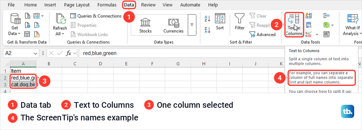
Open the Data tab and select Text to Columns in the Data Tools group. Its ScreenTip on our PC used names as its example, saying you can separate a column of full names into separate first and last name columns. It also listed the two ways to split, fixed width or at each comma, period or other character.
The Convert Text to Columns Wizard opens at Step 1 of 3, and ours already had Delimited selected with the line "The Text Wizard has determined that your data is Delimited." It said the same for codes like AB1234 that contain no separator at all, so check the choice rather than trusting it. Select Next.
Step 2 lists the delimiters. By default only Tab was ticked, so tick the character your text really uses, such as Comma or Space, and watch the Data preview draw a line at each split. When parts are separated by a comma and a space, tick both Comma and Space, as Microsoft suggests, and tick Treat consecutive delimiters as one, which its help describes for a separator of more than one character. Then check the preview shows no empty column.
Step 3 sets the format of each new column and where the results go. General was selected by default, and Destination defaulted to $A$2, the first cell of our original text, which means Finish would write the first part over the original. We typed $B$2 instead and selected Finish.
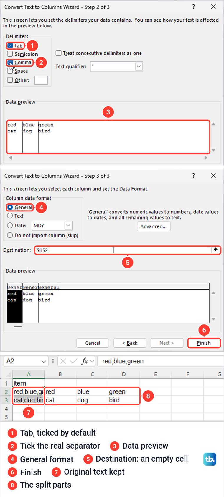
On our sheet red,blue,green and cat,dog,bird turned into red, blue and green in B2:D2 and cat, dog and bird in B3:D3, with the original text still in column A. Once the split looks right, you can move the finished columns in Excel to wherever they belong.
Text pasted from a PDF needs more care, because splitting on every space also breaks names and headings apart. If that is where your data came from, our guide to convert a PDF table to Excel is the better starting point.
Stop a split from overwriting your data
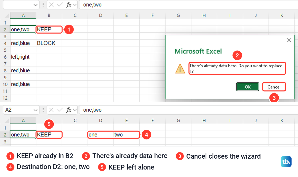
Text to Columns writes one column for every part it finds, and it writes into whatever cells are there. To see what happens, we put one,two in A2 and the word KEEP in B2, then ran a comma split with the Destination left at A2. Excel stopped and asked "There's already data here. Do you want to replace it?"
OK replaces the cells. Cancel closed the whole wizard on our PC and left the sheet unchanged, so every setting had to be chosen again from Step 1. With the Destination changed to D2, an empty cell, the split wrote one in D2 and two in E2, and KEEP stayed in B2.
The safest habit is to choose a Destination with as many empty columns to its right as there are parts. If your columns are full, insert blank columns first, as Microsoft recommends, and run the split into them.
How to separate names in Excel into first and last name
There are three good ways to separate first and last names. Flash Fill is the quickest to set up, Text to Columns with Space suits a long list where every name has two words, and formulas suit a list that will keep changing.
Separate names with Flash Fill
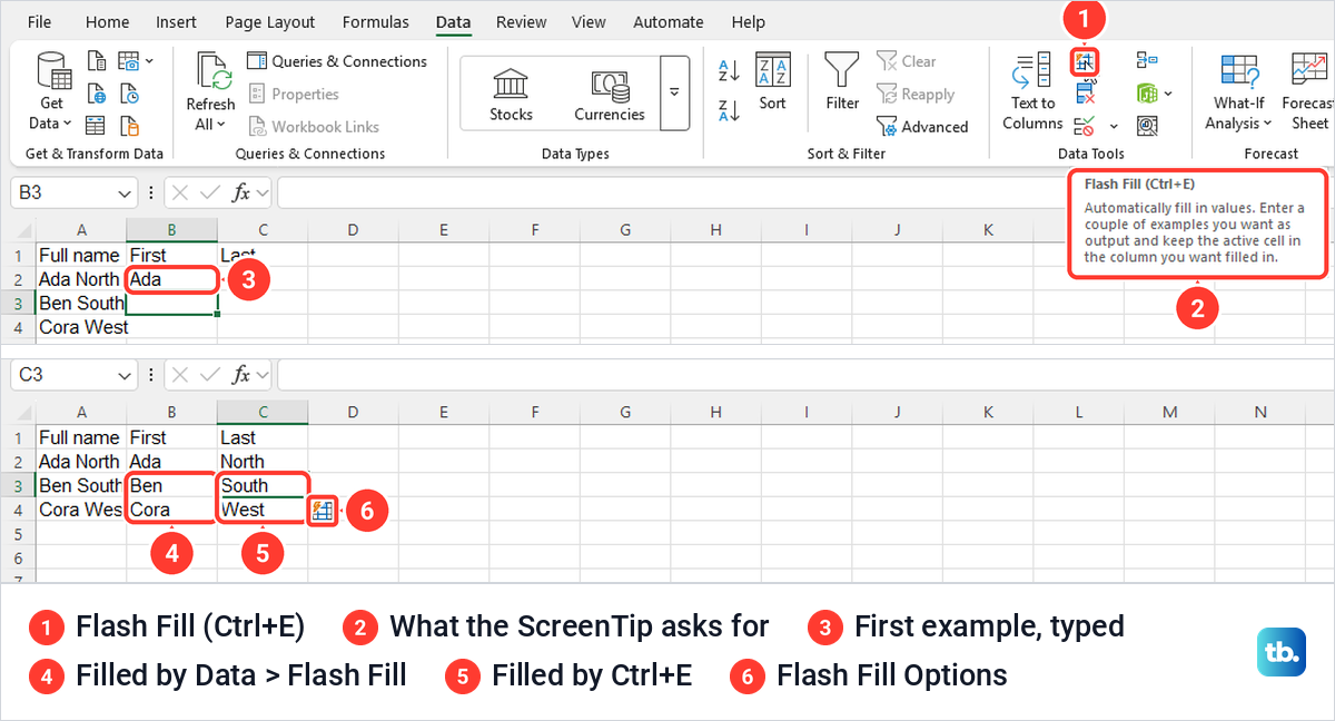
Put the full names in column A and add headings such as First and Last in B and C. On our sheet, with Ada North, Ben South and Cora West in A2:A4, we typed Ada in B2, selected B3 and chose Data > Flash Fill. Excel filled Ben and Cora at once.
On our screen the Flash Fill button was a small icon without a label in the Data Tools group, and its ScreenTip read "Flash Fill (Ctrl+E)". We typed North in C2, selected C3 and pressed Ctrl + E, which filled South and West. A Flash Fill Options button appeared beside the filled cells each time.
Do not wait for Excel to guess. Microsoft's Flash Fill page says that if Flash Fill does not show a preview, it might not be turned on. On our PC Automatically Flash Fill was ticked under File > Options > Advanced, yet typing Ben under Ada showed no preview and pressing Enter filled nothing. Pressing Ctrl + E then filled the rest straight away.
Separate names with Text to Columns
Follow the Text to Columns steps above, tick Space in Step 2 and clear the other boxes, which is what Microsoft suggests for names. Pick an empty Destination with two blank columns beside it.
Every space is a split point, so a name with three words fills three columns. Microsoft's own name examples point out that when a name has a middle name, the last name begins after the second space. Two-word surnames are split too, so look down the results and fix those rows by hand.
Separate names with a formula
Formulas work in every current version of Excel and update when a name changes. With Ada North in A3, =LEFT(A3,SEARCH(" ",A3)-1) returned Ada and =RIGHT(A3,LEN(A3)-SEARCH(" ",A3)) returned North on our sheet, and both returned the same results in Excel for the web.
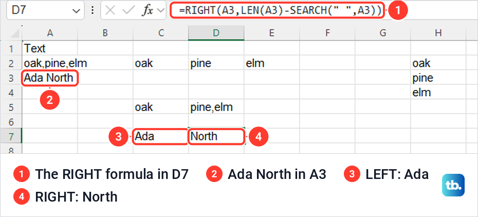
Both formulas split at the first space, so a middle name lands in the last-name result. If names still carry stray spaces after the split and TRIM does not remove them, our guide can help you fix the TRIM function when spaces remain. And if you need the full name back later, you can combine two columns in Excel with one formula.
Split codes at a fixed position
Some values have no separator, only a fixed layout, such as product codes where the first two characters are letters. In Step 1 of the wizard choose Fixed width instead of Delimited and select Next.
Step 2 shows a ruler above the preview and explains the controls itself. To create a break line, click at the position you want, double-click a line to delete it, and drag a line to move it. One click after the second character put a break between AB and 1234 on our sheet.
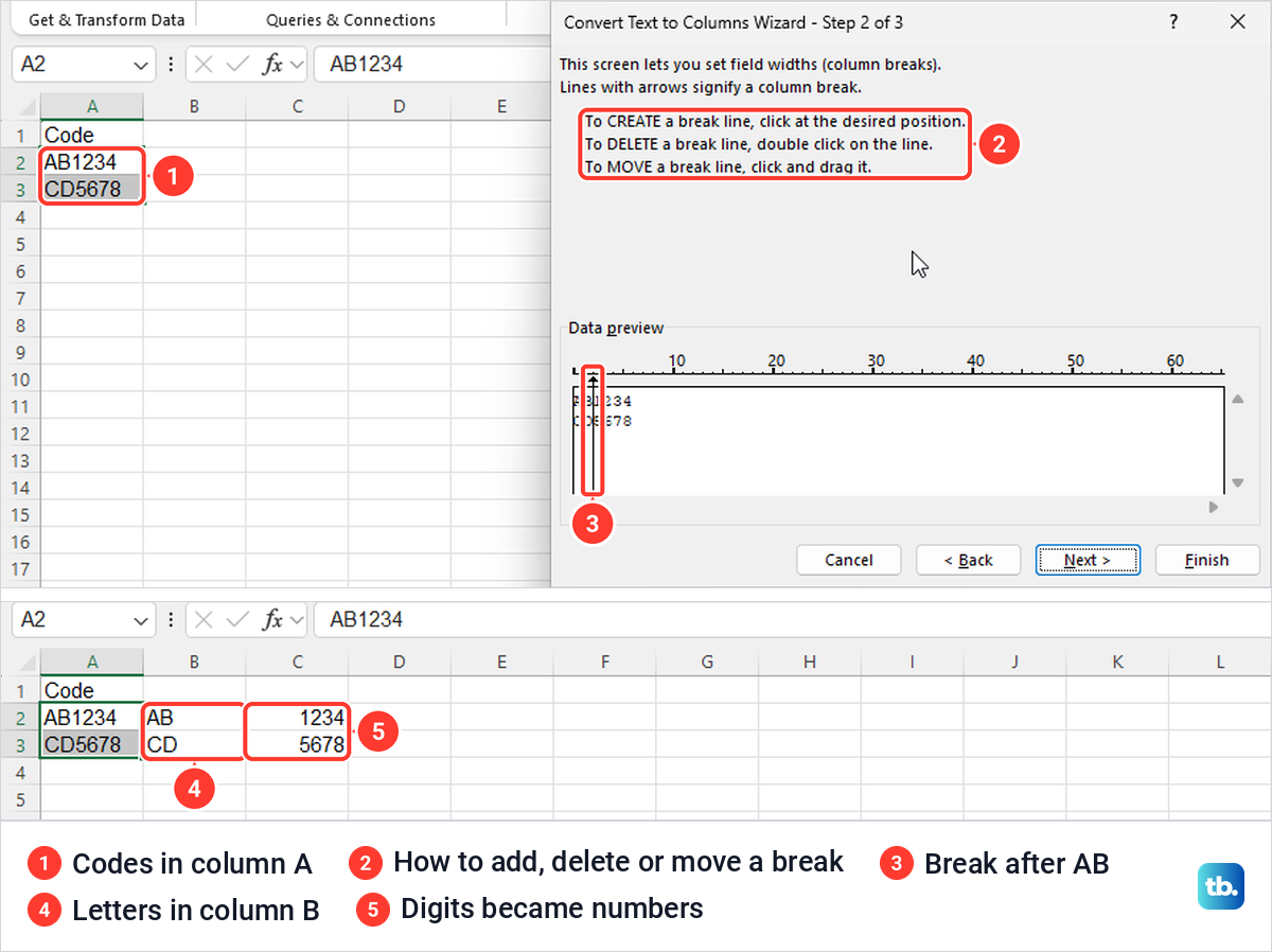
In Step 3 we set the Destination to B2, an empty cell, so the codes stayed in column A. After Finish, AB went to B2 and 1234 to C2, and the digits sat on the right of the cell because Excel had turned them into numbers under the General format. Microsoft warns that Excel automatically removes leading zeros from numbers, so a code such as 0042 would lose its zeros.
To keep them, click that column in the Step 3 preview and choose Text before you select Finish. Power Query also offers a By Number of Characters split for the same kind of data.
Split text with the TEXTSPLIT formula
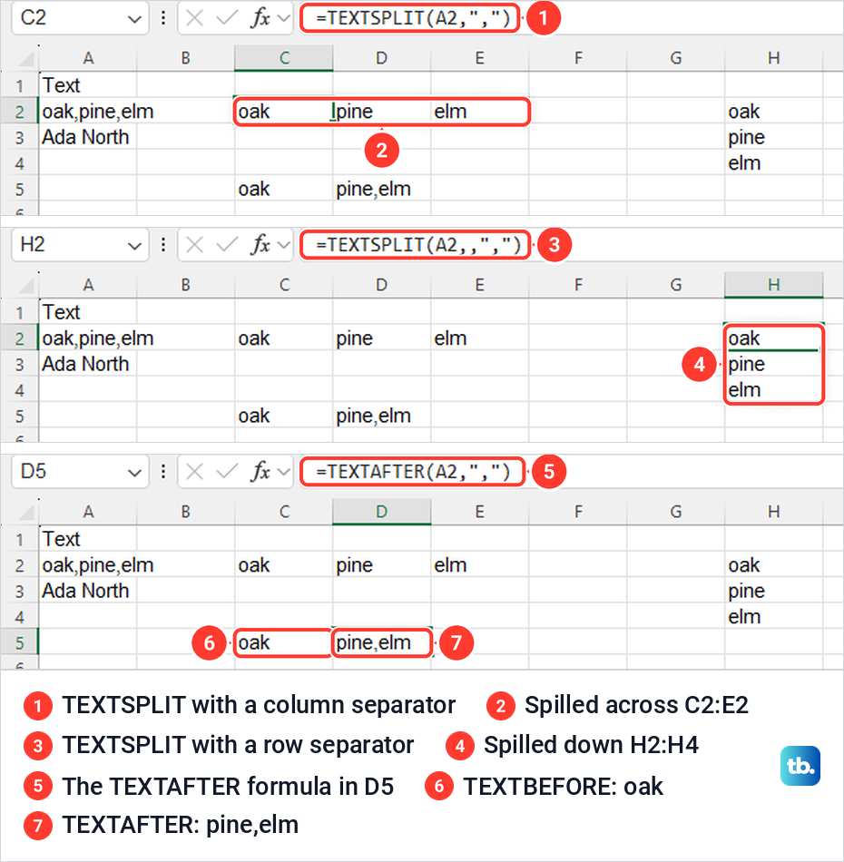
Text to Columns types fixed values, so if the original text changes, the split does not. TEXTSPLIT is a formula, so it keeps the original and updates with it. On our sheet, with oak,pine,elm in A2, =TEXTSPLIT(A2,",") typed in C2 spilled oak, pine and elm across C2:E2, with a blue border around the spill range.
To split down a column instead, leave the second part empty and give the separator as the third. =TEXTSPLIT(A2,,",") in H2 spilled oak, pine and elm down H2:H4. Leave enough empty cells in the direction of the spill, or the formula shows an error, as covered further down.
Doubled separators leave gaps by default. =TEXTSPLIT("a,,b",",") returned a, an empty cell and b, while =TEXTSPLIT("a,,b",",",,TRUE) returned just a and b, because TRUE in the fourth place tells Excel to ignore empty parts.
Take only the first part or the rest
When you only need one piece, TEXTBEFORE and TEXTAFTER are simpler. =TEXTBEFORE(A2,",") returned oak, and =TEXTAFTER(A2,",") returned pine,elm, which is everything after the first comma.
Microsoft lists TEXTSPLIT, TEXTBEFORE and TEXTAFTER for Excel for Microsoft 365 and Excel 2024, and TEXTSPLIT also worked in Excel for the web when we tried it. In an older version, Text to Columns gives the same split as fixed values and Flash Fill handles patterns such as names; the LEFT and RIGHT formulas only suit two-part names with one space. If a newer version still rejects the function, our steps to fix Excel functions that do not work can help.
If the cell shows =TEXTSPLIT(A2,",") as plain text instead of a result, follow our guide to fix formulas showing as text. It goes through the causes one at a time. And if a split formula stops updating after its source changes, check how to fix Excel formulas that stop updating.
Repeat the same split with Power Query
If the same messy column arrives every week, Power Query can save the split as steps you rerun. Select the range and choose Data > From Table/Range, which was an unlabelled icon in the Get & Transform Data group on our screen. Its ScreenTip says data that is not already a table will be converted into one.
The Create Table box opened with My table has headers unticked for our Code column, even though Code was a heading. Tick it when your first row is a heading, so Power Query does not treat that row as data, then select OK.
In the Power Query Editor, choose Home > Split Column > By Delimiter. The menu also offers By Number of Characters, By Positions and splits between lowercase and uppercase or digits and other characters. For our codes, AA-11 and BB-22, the dialog came pre-set to a custom hyphen delimiter and Each occurrence of the delimiter.
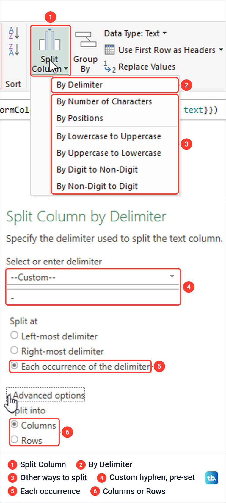
Under Advanced options you can choose Rows instead of Columns. Microsoft's Power Query help says the result then has the same number of columns but many more rows, one for each part.
Selecting OK gave us Code.1 with AA and BB, and Code.2 with 11 and 22. Power Query also added a Changed Type step that turned Code.2 into whole numbers, and changing numbers to text later cannot bring back zeros that are already gone.
If the digits must keep leading zeros, select Changed Type1 under Applied Steps, select Code.2, choose Home > Transform > Data Type > Text and select Replace Current, which is how Microsoft's leading-zeros help does it. Then check that Code.2 shows the zeros your original codes had.
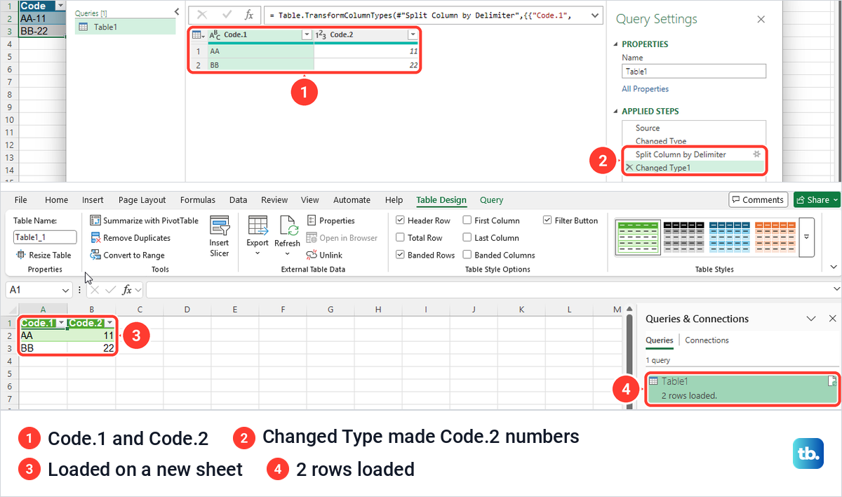
Home > Close & Load put the split as a new table on a new sheet, and the Queries & Connections pane showed "2 rows loaded". Microsoft says that when the source data changes, Data > Refresh updates the table and applies the same steps again.
Split text to columns in Excel for the web
Microsoft's split-cell help says Excel for the web does not have the Text to Columns Wizard and points to formulas instead. That is true of the wizard, but our Excel for the web had a different tool. In Editing mode, Data > Data Tools > Split Text to Columns opened a card with Tab, Semicolon, Comma, Space and Custom buttons, a preview and an Apply button.
The card has no Destination box, and that matters. Applying Comma to one,two in A11 turned A11 into one and wrote two in B11, so the original text was gone. Copy the column to an empty part of the sheet first, run the split on the copy, and make sure the columns to its right are empty.
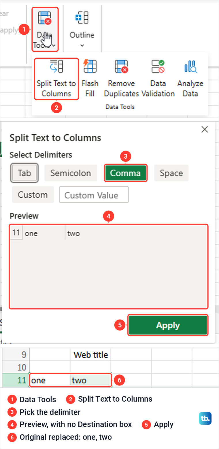
If Split Text to Columns is greyed out, check the mode button near the top right. Ours offered Editing and Viewing, and in Viewing the sheet showed "You're viewing live updates in View Mode" while Split Text to Columns, Flash Fill and Remove Duplicates were all greyed out. Switch back to Editing and they work again.
The formulas work in a browser as well. In Excel for the web, =TEXTSPLIT(A2,",") spilled red, blue and green across C2:E2, and =TEXTSPLIT(A3,,",") spilled oak, pine and elm down H2:H4.
Unmerge a cell that was merged
If the cell you want to split is really several cells merged into one, unmerge it. Select it, open the Home tab and select the small arrow beside Merge & Center in the Alignment group, then choose Unmerge Cells. On our sheet the button was an icon without a label, and its ScreenTip read "Merge & Center".
Our merged B2:C2 became two separate cells again, and the text "Merged title" stayed in B2, the upper-left cell. While a cell is being edited, the whole Alignment group is greyed out, so press Esc first if the arrow does nothing.
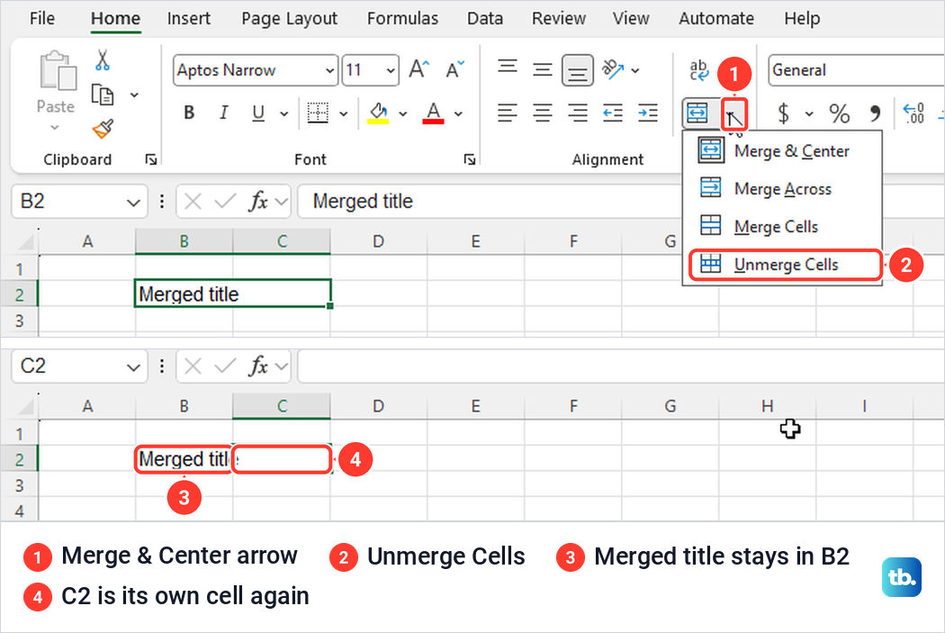
Unmerging does not bring anything back. Microsoft says the contents of the other cells that you merge are deleted, so before you merge cells again, see how to merge cells in Excel without losing data. If a whole sheet is full of merged areas, our guide to unmerging cells in Excel shows how to find and separate them.
Excel for the web works the same way. The arrow beside the Merge & Center icon opened a Merge & Unmerge Cells menu with Unmerge Cells at the bottom, and our merged B9:C9 split back into two cells with "Web title" in B9.
Fix a split that Excel blocks
A TEXTSPLIT formula needs every cell in its spill range to be empty. When we left the word BLOCK in E4 and typed =TEXTSPLIT(A4,",") in D4, the cell showed #SPILL! with a dashed outline around the cells it wanted. The error button's ScreenTip read "A cell we need to spill data into isn't blank."
Open that error button and choose Select Obstructing Cells. Excel selected E4 for us, and once we cleared BLOCK, red and blue appeared in D4:E4. If the cell holds something you need, move the formula to an empty area instead.
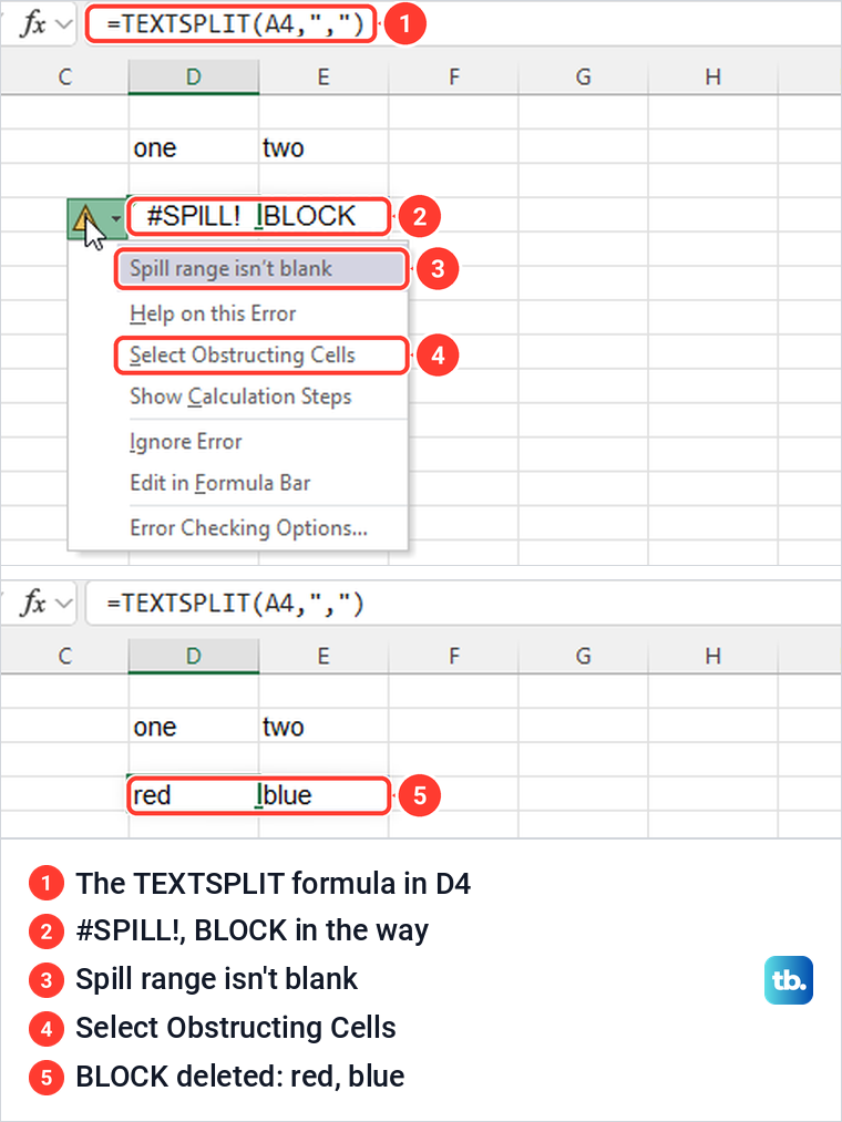
A merged cell blocks a spill too. With E6:F6 merged, the same kind of formula showed #SPILL! with the ScreenTip "We can't spill into a merged cell.", and Unmerge Cells fixed it. Microsoft adds that spilled formulas are not supported inside Excel tables, so move the formula outside the table or use Table Design > Convert to Range.
If Text to Columns is greyed out on the desktop, the sheet may be protected. On our protected sheet the Review tab showed Unprotect Sheet and Text to Columns was grey, and clicking it did nothing, with no message at all.
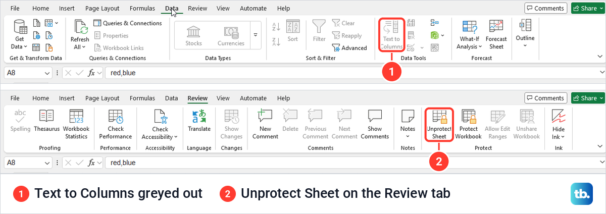
Select Review > Unprotect Sheet, entering the password if the sheet has one. After that, the same comma split worked on our sheet and wrote red and blue into D8:E8.
How we tested this guide
We tested this in Excel for Microsoft 365 on Windows 11, version 25H2, and in Excel for the web in Microsoft Edge, splitting made-up names and comma-separated lists.
Frequently Asked Questions
Can I split one Excel cell in half?
No. Excel cannot divide one ordinary cell into two smaller cells, so you split its contents into the cells beside it with Text to Columns, Flash Fill or TEXTSPLIT. If the cell was merged earlier, Unmerge Cells separates it again.
How do I separate first and last names in Excel?
Type the first name beside the first full name, select the cell below and press Ctrl + E, then repeat for the last name. For a long list of two-word names, Text to Columns with Space and an empty Destination also works. Check any name with more than two words.
Does Text to Columns overwrite the original cell?
It can. The desktop wizard used the original cell as its Destination by default on our PC, so change it to an empty cell before Finish. The web card has no Destination and replaced the original text, so split a copy there.
How do I split text into rows instead of columns?
Use =TEXTSPLIT(A2,,",") in an empty cell with empty cells below it. In Power Query, choose Rows under Advanced options in the Split Column by Delimiter dialog.
Why does TEXTSPLIT show #SPILL!?
A cell in the spill range is not empty or is merged. Use the error button's Select Obstructing Cells to find it, then clear or unmerge it, or move the formula. Inside an Excel table, move the formula out of the table.
Why is Text to Columns greyed out?
On the desktop, check whether the sheet is protected and use Review > Unprotect Sheet if it is. In Excel for the web, switch the mode button from Viewing to Editing.
Why does Flash Fill not fill anything?
Excel may not show a preview even when Automatically Flash Fill is on, as happened on our PC. Type one example, select the next cell down and press Ctrl + E or choose Data > Flash Fill.