
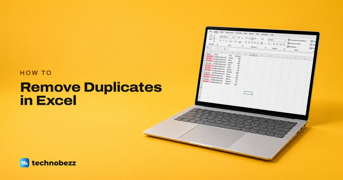
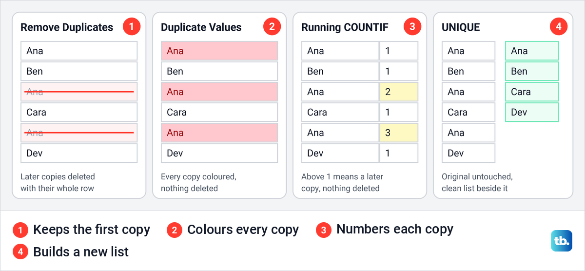
To remove duplicates in Excel, click any cell in your list, open the Data tab and select Remove Duplicates in the Data Tools group. Leave My data has headers ticked, tick the columns that together make a row a repeat, and select OK. Excel deletes the later copies, keeps the first one and tells you how many it removed. To find duplicates without deleting anything, select the column and choose Home > Conditional Formatting > Highlight Cells Rules > Duplicate Values.
Two details decide whether that goes well. Remove Duplicates deletes the whole row, including columns you left unticked, and the highlight colours every copy, the first one included, so never delete everything that turns red. Copy the sheet first, or build a clean list beside the original with the UNIQUE function.
We ran Remove Duplicates, the highlight, COUNTIF and UNIQUE in Excel for Microsoft 365 on Windows 11, version 25H2, on a made-up contact list with repeats planted on purpose. Three results are worth knowing before you start: Excel ignored capital letters, it did not ignore a trailing space, and the highlight and Remove Duplicates disagreed about numbers and dates.
The short version
- Delete repeats: click a cell in the list, choose Data > Remove Duplicates (or press Alt, A, M), tick the columns that define a repeat and select OK. Excel keeps the first copy.
- Find them first: Home > Conditional Formatting > Highlight Cells Rules > Duplicate Values colours every copy, the first one too.
- Count them: =COUNTIF($A$2:$A$13,A2) in a spare column shows how often each entry appears.
- Keep the original: =UNIQUE(A2:A13) writes a clean list beside it in Microsoft 365, Excel 2024, Excel 2021 and the web.
- Changed your mind: press Ctrl + Z straight away.
Pick the right way to deal with duplicates
Excel has one command that deletes repeats and several ways to find them without touching your data. Choose by what you want to end up with: a shorter list, a list with the repeats marked, or a clean copy next to the original.
| Method | What it does | Where to find it | Keeps your original data? | In Excel for the web |
|---|---|---|---|---|
| Remove Duplicates, Alt, A, M | Deletes later copies and keeps the first | Data > Data Tools > Remove Duplicates | No, it deletes whole rows | Yes |
| Duplicate Values highlight | Colours every copy, the first included | Home > Conditional Formatting > Highlight Cells Rules | Yes, it only colours cells | Yes |
| COUNTIF formula | Counts each entry or numbers its copies | A formula in a spare column | Yes, it adds a column | Yes |
| UNIQUE formula | Writes a clean list somewhere else | =UNIQUE(A2:A13) in an empty cell | Yes | Yes |
| Advanced Filter | Copies unique rows to a new place | Data > Sort & Filter > Advanced | Yes, it copies | No Advanced button |
| Data Validation rule | Refuses a repeat as it is typed | Data > Data Validation > Custom | Yes | Yes |
Here, a duplicate means a row that matches another row on the columns you choose, not just one matching cell. Microsoft adds that the comparison depends on what the cell shows rather than the value stored underneath, which matters for numbers and dates.
Remove duplicates in Excel on Windows
Microsoft describes removing duplicates as permanently deleting them, so make a copy of the workbook, or at least of the sheet, before you start. For a sheet, right-click its tab, choose Move or Copy, tick Create a copy and select OK. That box was unticked by default on our PC, and Excel named the copy Contacts (2).
Click any cell inside the list, then open the Data tab. On our screen the Data Tools group showed small icons, and only Text to Columns kept its label. Remove Duplicates was the middle icon in the column just right of Text to Columns, between Flash Fill and Data Validation, and hovering over it showed the tooltip "Remove Duplicates" with "Delete duplicate rows from a sheet."
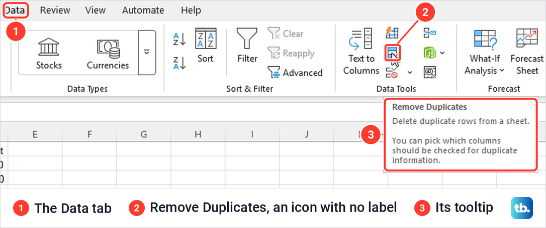
The keyboard is quicker. Press and release Alt, then A for the Data tab, then M, and the Remove Duplicates dialog opens. Those are the Key Tips Excel showed on our screen, and you can learn other Excel keyboard shortcuts the same way, by pressing Alt and reading the letters.
With one cell selected, the dialog picked up the whole list by itself. Leave My data has headers ticked if row 1 holds column names, so the boxes under Columns carry those names. With it unticked, the list read Column A to Column D and row 1 was treated as data.
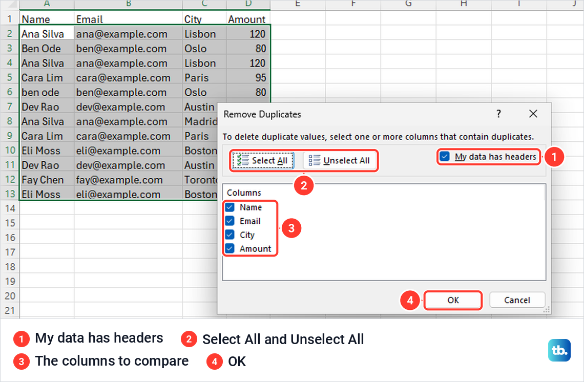
Select All ticks every column and Unselect All clears them, which is the fast way to tick just one or two. With every column ticked, a row goes only when it matches another row in every column. Select OK when the ticks are right.
Excel answered with a message: "4 duplicate values found and removed; 8 unique values remain. Note that counts may include empty cells, spaces, etc." The first Ana Silva row stayed, the rows below moved up to close the gaps, and a lower-case copy of Ben Ode was one of the four that went.
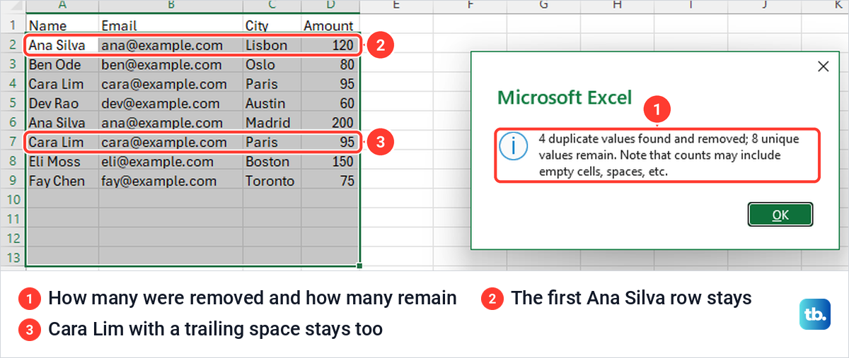
Changed your mind? Press Ctrl + Z straight away. On our PC one press brought all 12 rows back exactly as they were.
If your list is an Excel table, the same command also sits on the Table Design tab in the Tools group, where it keeps its label. On our table it opened the same dialog and gave the same message, and its Key Tips were Alt, J, T, M.
Choose the columns that make a row a duplicate
The ticks under Columns choose what Excel compares, not what it keeps. Microsoft puts it plainly: data will be removed from all columns, even if you do not select all the columns. When two rows match on the ticked columns, the entire later row goes, unticked columns included.
Our list has a third Ana Silva row with the same email but a different city, Madrid, and a different amount. With only Name and Email ticked, Excel removed five rows instead of four, and the Madrid row went with its city and amount. Unticking City did not protect it; it only told Excel to ignore City when looking for matches.
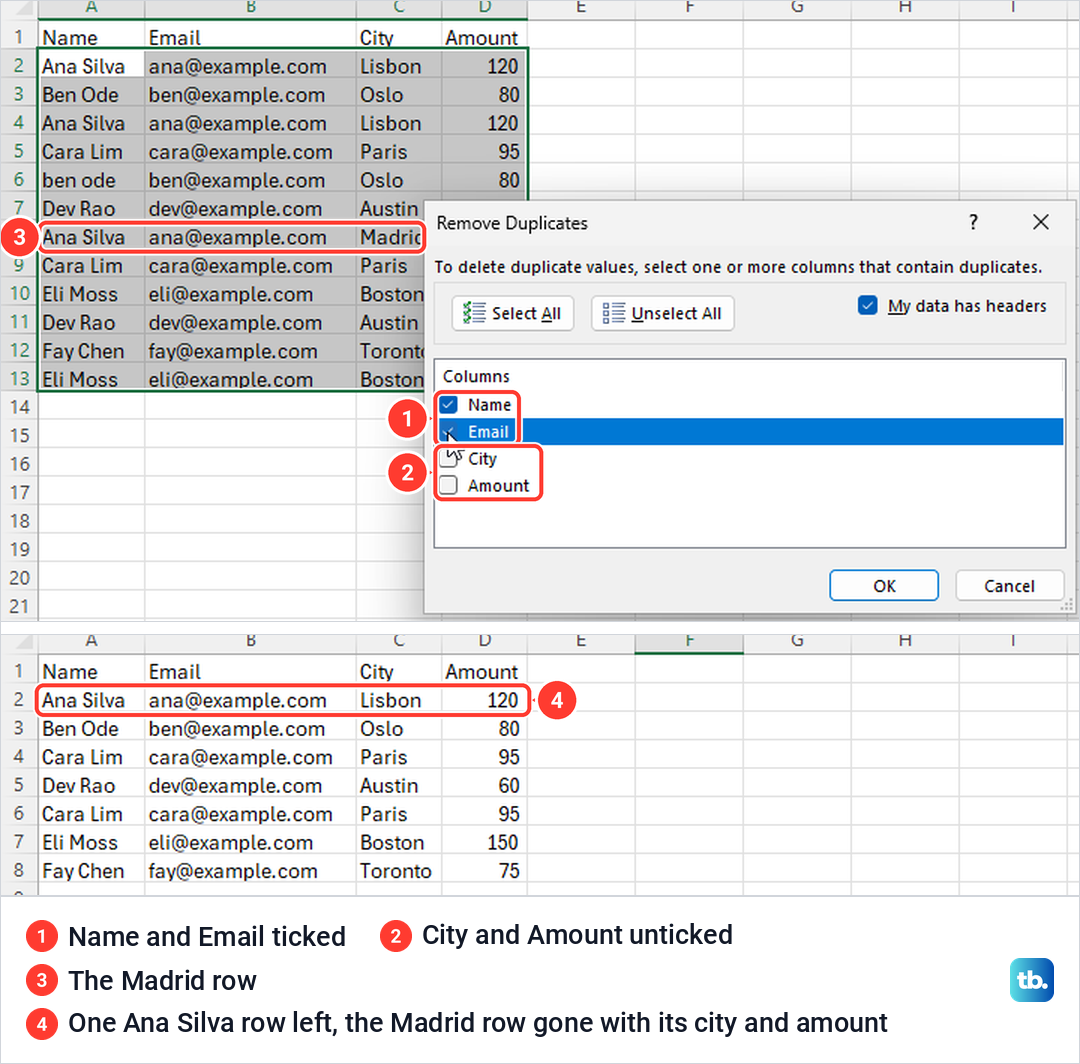
So tick every column that has to match for two rows to be the same record. If two orders from one customer have different amounts and both matter, leave Amount ticked, or the second order disappears. One example on Microsoft's own find-and-remove page reads as if unticking a column keeps its data, but on our screen the whole row went.
Select the whole list, or a single cell in it, rather than one column. When we selected only the Name column, Excel stopped with a Remove Duplicates Warning: "Microsoft Excel found data next to your selection. Because you have not selected this data, it will not be removed."
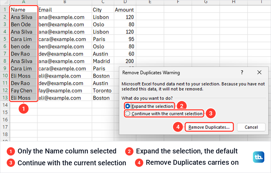
Expand the selection is chosen by default, and it is the one you want: leave it chosen and select Remove Duplicates to carry on. Continue with the current selection cleans that column on its own while the cells beside it stay where they are, so the names left behind can end up next to the wrong email and city. When we chose it, the next dialog listed only Column A, with My data has headers unticked.
Find duplicates in Excel with the Duplicate Values highlight
To see repeats without deleting anything, select the column, open Home > Conditional Formatting > Highlight Cells Rules and choose Duplicate Values. The dialog has two boxes, set to Duplicate and to Light Red Fill with Dark Red Text by default. Select OK, or pick another colour first.
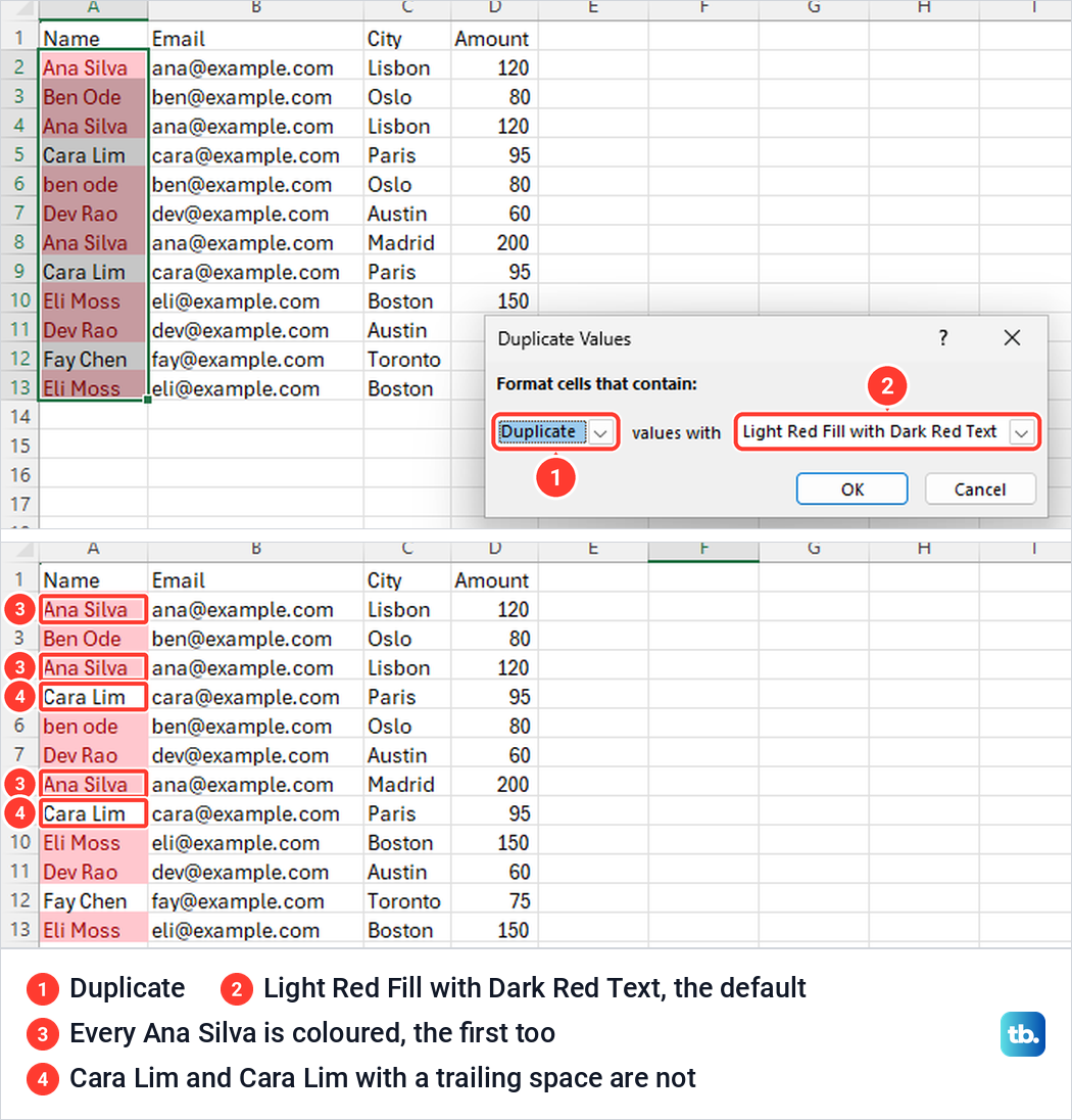
Now look at what got coloured. All three Ana Silva cells turned red, the first one too, because this rule marks every copy rather than only the extra ones. Delete every coloured row and you lose the originals along with the repeats, so use the colour to review, then run Remove Duplicates.
The rule ignored case but not spaces. Ben Ode and ben ode were both coloured, while Cara Lim and a Cara Lim typed with a trailing space were not, even though the two look identical. From the keyboard, Alt, H, L, H, D opened the same dialog for us.
On a long list, freeze the header row so the column names stay in view while you scroll through the colours. When you are done, Home > Conditional Formatting > Clear Rules removes the rule from the selected cells or the entire sheet. If a colour is missing where you expect one, check for a trailing space, covered below, and our guide to conditional formatting not working in Excel walks through the fixes.
Find and count duplicates with COUNTIF
A formula gives you numbers you can sort and filter. In an empty column beside the list, type a heading such as Count in row 1, then =COUNTIF($A$2:$A$13,A2) in row 2, and fill it down using your own range. Each row then shows how many times its entry appears in the whole column, which was 3 for each Ana Silva and 1 for a name that appears once.
Lock only the start of the range, =COUNTIF($A$2:A2,A2), and the count numbers the copies instead. Our first Ana Silva showed 1, the second 2 and the third 3, so any row above 1 is a later copy. That makes it easy to sort or filter the extra copies before you delete anything.
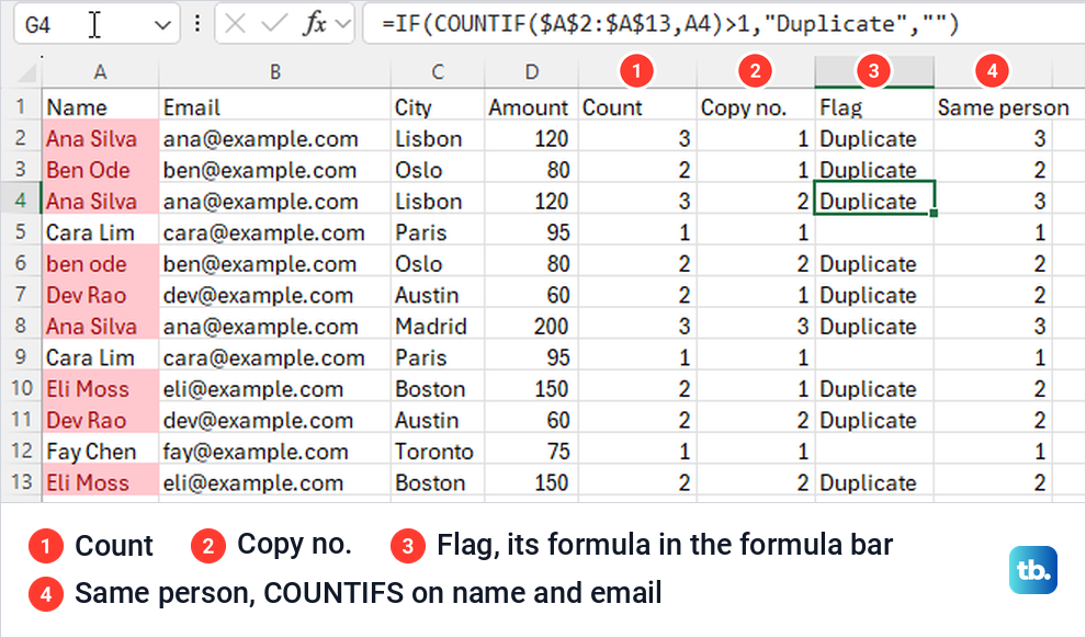
To see a word instead of a number, wrap the count in an IF statement: =IF(COUNTIF($A$2:$A$13,A2)>1,"Duplicate","") labels every copy, the first included. For rows that must match on two columns, COUNTIFS takes a range and a value for each one, as in =COUNTIFS($A$2:$A$13,A2,$B$2:$B$13,B2) for name plus email.
COUNTIF behaved like the highlight on our list. It counted ben ode together with Ben Ode, ignoring capitals as Microsoft says it does, and it counted the Cara Lim with a trailing space as a different name.
To delete every copy of a repeated entry, the first included, turn on Data > Filter, open the arrow on the Count column, the one with =COUNTIF($A$2:$A$13,A2) rather than the running count, and choose Number Filters > Greater Than, then enter 1. Select the row numbers of the visible rows below the header, right-click and delete those rows, then clear the filter. What is left are the entries that appeared only once.
The same idea compares two lists. Select the first list starting at A2, so that A2 is the active cell, choose Home > Conditional Formatting > New Rule > Use a formula to determine which cells to format, enter =COUNTIF(List2!$A$2:$A$500,A2)>0 and pick a format. It colours names that also appear on the List2 sheet, since Microsoft says a formula rule can look at another worksheet in the same workbook.
Colour only tells you that a name is in both lists. To pull the matching details with XLOOKUP, look each name up in the other sheet, and to match on one column instead of two, combine two columns into one first.
Make a clean copy with the UNIQUE function
UNIQUE leaves your data alone and writes a clean list somewhere else. Click an empty cell to the right of the list, type =UNIQUE(A2:A13) with your own range and press Enter. The result spills down as many rows as it needs, and a thin blue border marks the spill area while one of its cells is selected.
On our list it returned seven names from twelve. Like Remove Duplicates, it treated ben ode as Ben Ode, and it listed Cara Lim twice because one copy carried a trailing space.
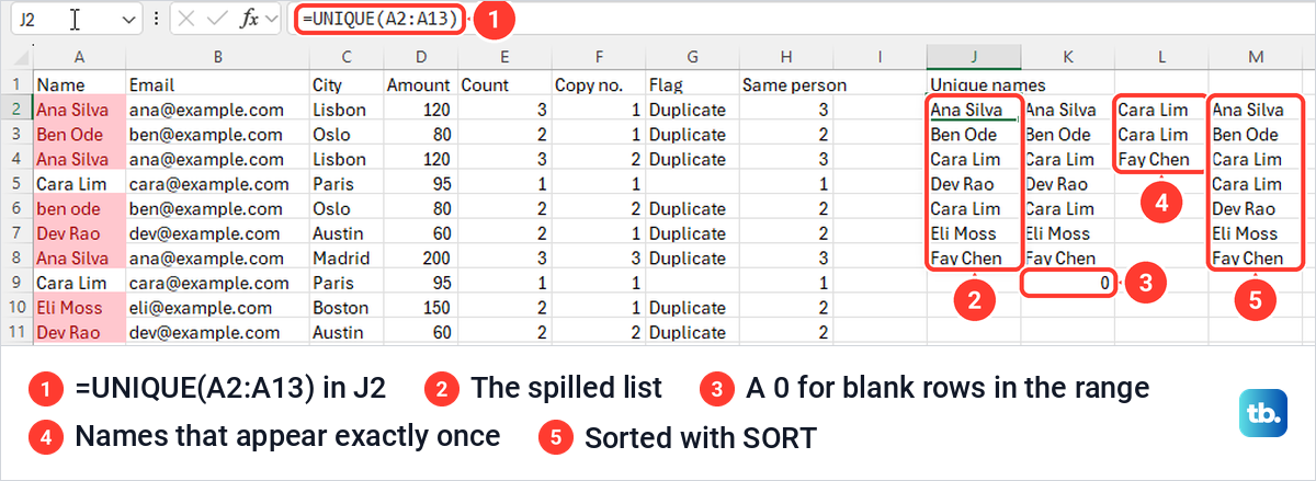
Three variations are worth knowing. =UNIQUE(A2:A13,,TRUE) lists only the entries that appear exactly once, =SORT(UNIQUE(A2:A13)) sorts the clean list, and =UNIQUE(A2:D13) compares whole rows across all four columns, which kept the Madrid row as its own record.
Leave blank rows out of the range. When we stretched it to A2:A15, with two empty rows at the end, the list gained a 0 at the bottom.
UNIQUE is a formula, so its list changes when the source changes. To keep it as fixed values, copy the result, click a different empty cell, press Ctrl + Alt + V and choose Values. Delete the UNIQUE formula only after the pasted values are in place.
Microsoft lists UNIQUE for Microsoft 365, Excel 2024, Excel 2021, Excel for the web, Mac, iPad, iPhone and Android, but not Excel 2019 or 2016. In those versions, select the list including its header row, then Data > Advanced makes a one-off copy instead: choose Copy to another location, enter a cell in the Copy to box, tick Unique records only and select OK.
Fix a #SPILL! error from UNIQUE
A spilled list needs empty cells to land in. When we typed an x into one of the cells UNIQUE was using, the formula cell turned into #SPILL!, a dashed border showed the area it wanted, and a warning icon appeared beside it. Deleting the x brought the list straight back.
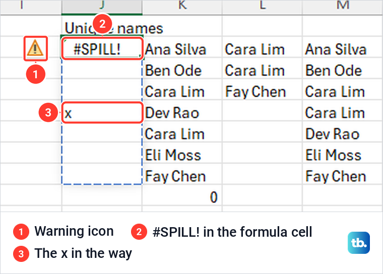
Microsoft's fix is to select that warning icon and choose Select Obstructing Cells, which jumps to whatever is in the way. Clear or move those cells and the list spills again.
Two other things stop a spill. Microsoft says spilled formulas are not supported inside Excel tables, so put UNIQUE in an empty cell beside the table, or turn the table back into a normal range with Table Design > Convert to Range. A spill cannot land in merged cells either, so unmerge the cells below the formula first.
Why Excel misses duplicates you can see
When Excel's count does not match what you can see, either the cells are not identical underneath or Excel is matching more loosely than you expect. On our test data, these five things explained the mismatches.
Capital letters do not count. Remove Duplicates, the highlight, COUNTIF and UNIQUE all treated ben ode as a copy of Ben Ode on our PC. If case matters to you, these tools cannot keep the two apart, and Microsoft says Power Query is case sensitive when it removes duplicates.
Extra spaces do count. A name typed with a space at the end is a different entry to every one of those tools. We added a helper column with =TRIM(A2), pasted it back as values, and ran Remove Duplicates on that column and Email. Six rows went instead of five, and the extra one was the Cara Lim copy with the trailing space.
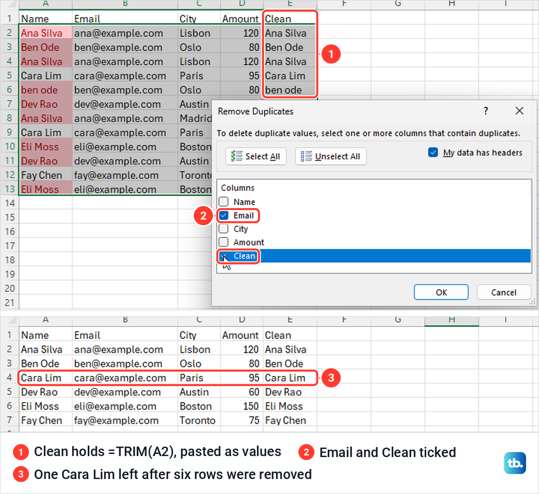
TRIM only removes the ordinary space character. Microsoft notes that web pages commonly use a nonbreaking space, character 160, which TRIM leaves alone. If TRIM leaves a space behind, Microsoft's answer is SUBSTITUTE, which can swap character 160 for an ordinary space first, as in =TRIM(SUBSTITUTE(A2,CHAR(160)," ")).
Remove Duplicates goes by what the cell shows. In a short column of test values, the number 1 shown as 1.00 and the number 1 shown as 1 both stayed, and so did one date shown in two formats. A formula that returned 1, =2-1, was removed as a copy of the plain 1, which matches Microsoft's description.
The highlight does not follow that rule. On the same cells it coloured all eight values, 1.00 and 1 alike and both dates. If the two tools report different numbers for your list, this is one reason, and another is that Remove Duplicates compares whole rows while the highlight checks single cells.
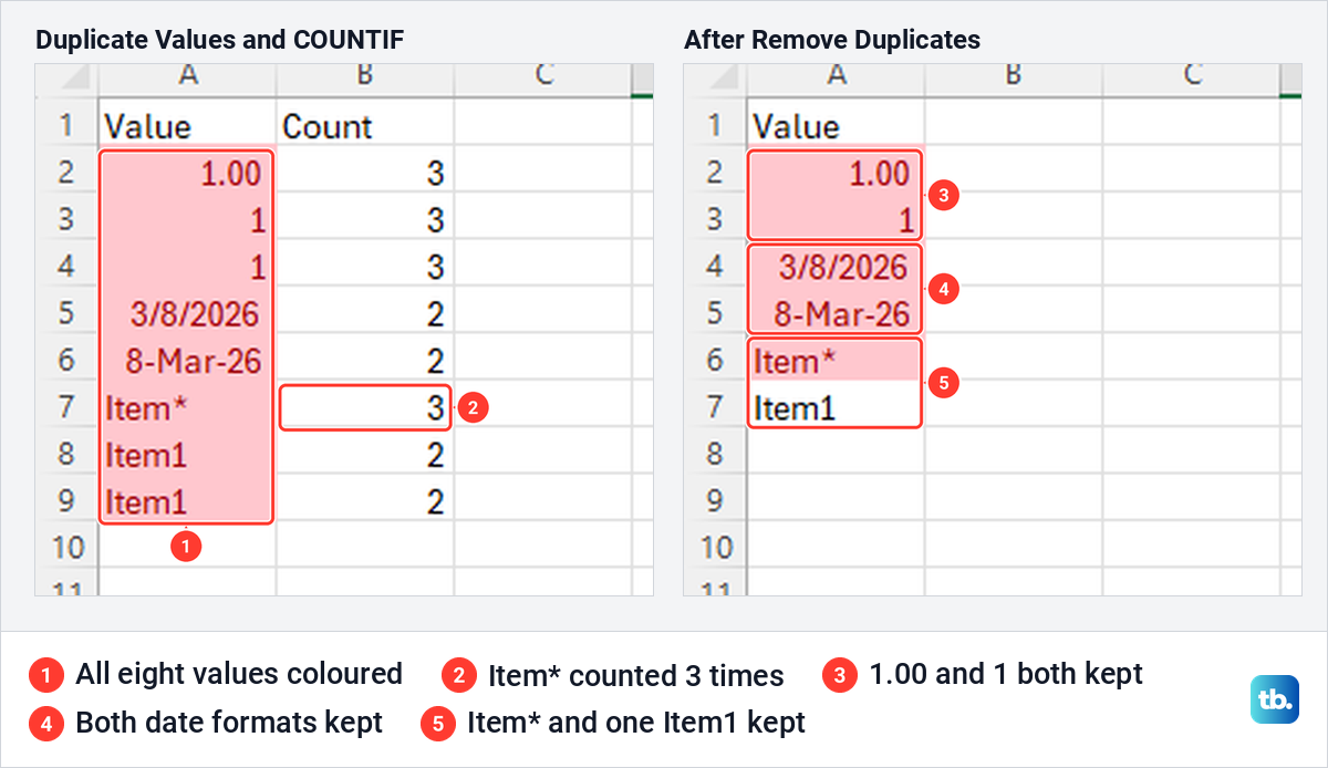
An asterisk acts as a wildcard. Item* was coloured as a duplicate, and COUNTIF counted it three times because it matched both Item1 cells as well as itself. Remove Duplicates kept Item* as its own entry, and Microsoft says a question mark acts as a wildcard in the highlight and COUNTIF too. On codes that contain an asterisk or question mark, treat a colour or a count as a hint, not proof.
Remove duplicates in Excel for the web
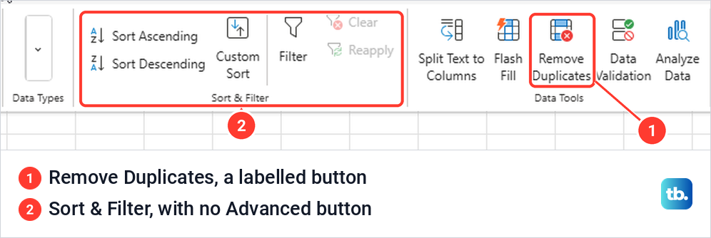
Excel for the web has the same command, and it is easier to spot. On our screen the Data tab showed Remove Duplicates as a labelled button in the Data Tools group, next to Split Text to Columns, Flash Fill, Data Validation and Analyze Data. At another moment the group was folded into a Data Tools menu that listed the same five commands, so look there if the button is missing.
The steps match the desktop. Select the range or a cell in a table, select Data > Remove Duplicates, untick any columns you do not want compared and select OK. A message says how many duplicate values were removed, and Ctrl + Z or Undo brings them back. Microsoft's warning carries over too: data is removed from all columns, even the ones you leave unticked.
To highlight repeats, select the cells and choose Home > Styles > Conditional Formatting > Highlight Cell Rules > Duplicate Values, which is how Microsoft's web instructions name the menu. Rules you add are managed in a Conditional Formatting pane rather than a dialog. UNIQUE works in the browser, and Microsoft says its COUNTIF validation rule works there too.
One desktop tool is missing. The Sort & Filter group on our screen had Sort Ascending, Sort Descending, Custom Sort, Filter, Clear and Reapply, with no Advanced button. Use UNIQUE when you want a clean copy in the browser.
Remove duplicates in Excel for Mac
In Excel for Mac, select the range or a cell in a table, then on the Data tab, in the Data Tools group, click Remove Duplicates. Tick the columns to compare, then, as Microsoft's Mac steps put it, click Remove Duplicates again rather than OK. To compare only a few columns of a wide table, Microsoft suggests clearing the Select All check box first.
The highlight is under Home > Conditional Formatting > Highlight Cells Rules > Duplicate Values, and Microsoft says you then pick the options in the New Formatting Rule dialog box. UNIQUE and COUNTIF are both listed for Excel for Mac, so the formula methods above work there too.
Stop duplicates being typed in
Once a list is clean, Data Validation can keep it that way. Select the cells people will type into, starting at the top so that A2 is the active cell, then open Data > Data Validation. Set Allow to Custom, enter =COUNTIF($A$2:$A$20,A2)=1 in the Formula box with your own range, and select OK.
We typed Ana Silva in A2, then typed it again in A3. Excel refused the second one with "This value doesn't match the data validation restrictions defined for this cell." and offered Retry and Cancel. Pressing Esc, which cancels, left the cell empty.
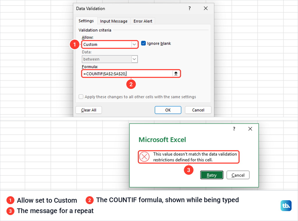
The rule lives in the same dialog you use to make a drop-down list in Excel, with Allow set to Custom instead of List. It has one gap: Microsoft says validation only checks what is typed into a cell, so values that are pasted or filled in get no message. Run Remove Duplicates again after a big paste.
Undo a removal or fix a greyed out button
Press Ctrl + Z as soon as you see a wrong result. Microsoft says undo still works after you save, as long as you are within the last 100 actions, but running a macro clears the undo list. Beyond that, go to your backup sheet, or restore an earlier version of the file if it is saved in OneDrive or SharePoint.
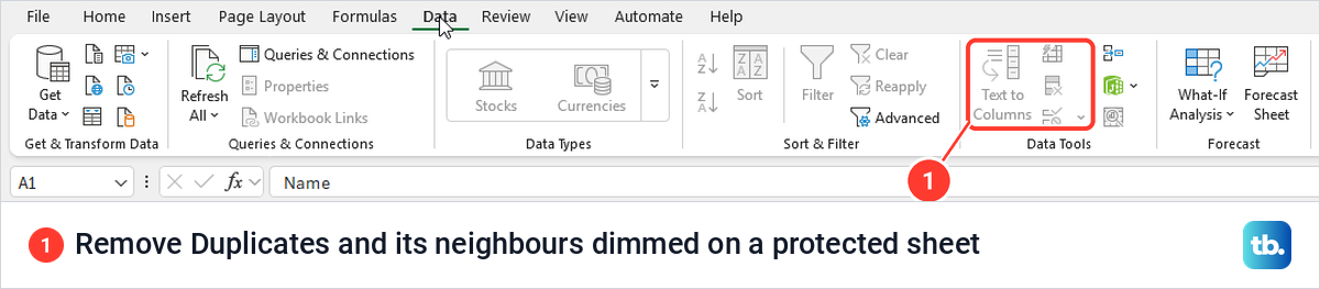
Remove Duplicates was greyed out on our PC in two situations. On a protected sheet it was dimmed along with Text to Columns, Flash Fill and Data Validation, so unprotect the Excel worksheet first. The whole Data Tools group was dimmed while a cell was still being edited, so press Enter or Esc to finish the entry.
Microsoft also says Remove Duplicates will not work on data that is outlined or has subtotals. Remove the subtotals and the outline first, then run it again.
Remove Duplicates always keeps the first copy it meets. To keep the newest record instead, sort the list so the copy you want comes first, for example by date from newest to oldest, then remove duplicates.
How we tested this guide
We ran Remove Duplicates, the Duplicate Values highlight, COUNTIF, COUNTIFS, UNIQUE, a TRIM helper column and a Data Validation rule in Excel for Microsoft 365 on Windows 11, version 25H2. The data was a made-up 12-row contact list with repeats planted on purpose, plus a short column of numbers, dates and codes in different formats.
We also opened the Data tab in Excel for the web to see where Remove Duplicates sits and what the Sort & Filter group offers. Every message quoted here was copied from the screen.
Frequently Asked Questions
Does Remove Duplicates keep the first or the last copy?
It keeps the first copy and deletes the later ones, which is what happened on every run we made. To keep a different copy, sort the list so that copy comes first, then remove duplicates.
Why does Remove Duplicates find a different number than the highlight?
Remove Duplicates compares whole rows on the ticked columns and leaves one copy, while the highlight checks single cells and colours every copy. Formats matter too: on our PC the highlight treated 1.00 and 1 as the same, but Remove Duplicates kept both.
Is removing duplicates in Excel case sensitive?
No. Remove Duplicates, the Duplicate Values highlight, COUNTIF and UNIQUE all treated ben ode and Ben Ode as the same name on our PC. Power Query is the exception, because Microsoft says it is case sensitive.
How do I delete every copy of a duplicate, including the first?
Add a COUNTIF column, filter it for values greater than 1 and delete the visible rows. Clear the filter afterwards, and only the entries that appeared once are left.
How do I find duplicates between two columns or two sheets?
Add a conditional formatting rule such as =COUNTIF(List2!$A$2:$A$500,A2)>0 to the first list, or =COUNTIF($C$2:$C$500,A2)>0 when the second list is column C of the same sheet. It colours every name that also appears in the other range, and XLOOKUP can then bring back the matching details.
Can I get my data back after removing duplicates?
Press Ctrl + Z right away, which restored all of our rows in one step. Microsoft says undo works even after a save within the last 100 actions, but a macro clears it, so keep a copy of the sheet for anything important.
Why is Remove Duplicates greyed out?
On our PC it was greyed out on a protected sheet and while a cell was still being edited. Microsoft adds that outlined data and subtotals must be removed before the command will work.