


To sum a column in Excel, click the empty cell below the numbers, select AutoSum on the Home tab, check the range Excel highlights and press Enter. Excel writes a formula such as =SUM(B2:B5) in that cell and shows the total. To choose the cells yourself, type the SUM formula instead, and to see a total without changing the sheet, select the numbers and read Sum on the status bar.
On our made-up column of 12, 8, 15 and 5, AutoSum proposed =SUM(B2:B5) and pressing Enter gave 40 in Excel for Microsoft 365 on Windows 11, version 25H2. If a total looks wrong, check for a blank cell that cuts AutoSum's range short, a number stored as text, a total already in the column, or a formula that refers to its own cell.
The short version
- Fastest: click the cell under the numbers, select Home > AutoSum, check the range and press Enter.
- Keyboard: Alt + = does the same job as the AutoSum button.
- Your own range: type
=SUM(B2:B5)in any empty cell outside the numbers. - No formula: select the numbers and read Sum on the status bar.
- Filtered lists: use a table Total Row or
=SUBTOTAL(109,E2:E5)to add only the visible rows. - Wrong total: look for a blank cell in the range, numbers stored as text and a total row counted again.
Pick the right way to sum a column
| Method | Do this | What you get |
|---|---|---|
| AutoSum on the Home or Formulas tab | Click the empty cell under the numbers, select AutoSum, check the range, press Enter | =SUM(B2:B5) in that cell, showing 40 |
| Alt + = | Press it in the empty cell under the numbers, then press Enter | The same formula and total as the button |
| Typed SUM formula | Type =SUM(B2:B5), or =SUM(B2:B3,B5:B6) for separate blocks | The total in any cell you choose |
| Whole-column SUM | Type =SUM(B:B) in a different column | Every number in column B, including any total typed there |
| Status bar | Select B2:B5 | Sum: 40 at the bottom of the window, with no formula added |
| Table Total Row | Table Design, then tick Total Row | A total under the table that follows filters |
| SUBTOTAL formula | Type =SUBTOTAL(109,E2:E5) in a row below the filtered list | A total of the visible rows only |
Our example list has 12, 8, 15 and 5 in B2:B5, so on the unfiltered list, with no total already in column B, every method here gives 40. Use a formula when the total has to stay in the workbook, and the status bar when you only want to check a number before you move on.
Sum a column with AutoSum
Click the first empty cell under the column, B6 in our example. On the Home tab, find the Σ button in the Editing group at the right end of the ribbon. Pointing at it showed the name Sum (Alt+=) and the line Automatically add it up.
One click put =SUM(B2:B5) in B6 straight away, with a moving dashed border round the cells it planned to add. This is the moment to check the range, because Excel picks it from the numbers next to the cell. If the border covers the right cells, press Enter, and if it does not, drag over the right cells first and the formula changes to match.
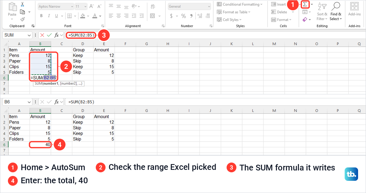
B6 then showed 40, and with B6 selected the formula bar showed =SUM(B2:B5). The total is a formula, not a typed number, so by default it updates when you edit one of the amounts in the range.
Microsoft notes that AutoSum is in two places, and the second is Formulas > AutoSum. The arrow under that button lists Sum, Average, Count Numbers, Max, Min and More Functions. Choosing Sum there proposed the same =SUM(B2:B5) and gave the same 40.
Use the AutoSum keyboard shortcut
Press Alt + = in the empty cell under the numbers. On our sheet it wrote the same =SUM(B2:B5) with the same dashed border, and Enter gave 40. It is the quickest route when your hands are already on the keyboard.
If you prefer the ribbon's key tips, press Alt, then H for the Home tab, U for AutoSum and S for Sum. Excel showed each letter on the ribbon as we went, and the last key produced the same formula. If you add up columns all day, keep this one with the other Excel keyboard shortcuts worth learning.
Type a SUM formula for the cells you choose
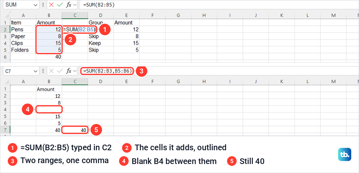
Typing the formula gives you full control of the range and lets you put the total anywhere. Click an empty cell outside the numbers, type =SUM(B2:B5) and press Enter. While you type, Excel outlines the cells the formula refers to, a quick check that you have the right rows. Our formula in C2 showed 40, and the formula bar showed it exactly as typed.
For numbers in separate blocks, list each range with a comma between them. With B4 left blank, =SUM(B2:B3,B5:B6) added 12, 8, 15 and 5 and gave 40. Plus signs work too, and =B2+B3+B4+B5 also gave 40, but a range is easier to read and to extend once a column has more than a few numbers.
A fixed range such as B2:B5 covers those cells and no others. If you need space for another amount, insert a row in Excel inside the range rather than under it, then check that the formula still covers the new cell.
Sum a whole column without counting the total twice
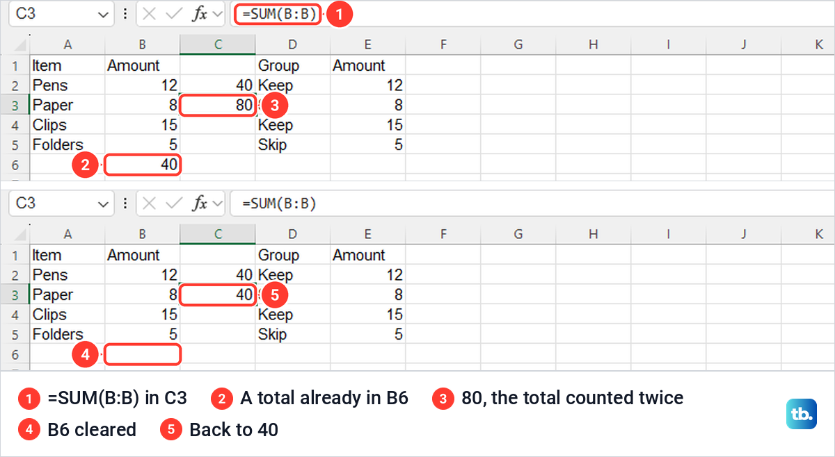
To total a column that keeps growing, refer to the whole column with =SUM(B:B) and put that formula in a different column. Microsoft describes its own example, =SUM(A:A), as adding all numbers in column A. That means every number, including a total you have already typed under the list.
That is exactly what happened on our sheet. With the AutoSum total of 40 still sitting in B6, =SUM(B:B) in C3 showed 80, because it added the four amounts and then their total. Once we cleared B6, the same formula showed 40.
So pick one approach per column. Either keep a bounded total such as =SUM(B2:B5) under the numbers, or keep the column clean and put =SUM(B:B) in a summary cell elsewhere. Never put =SUM(B:B) inside column B itself, because that makes a circular reference, covered in the fixes below.
A total that is too high can also come from the same record entered twice. If that is the cause, remove duplicate rows in Excel after checking which records should stay.
See the sum on the status bar without a formula
When you only need to check a number, select the cells and look at the bottom right of the Excel window. With B2:B5 selected, our status bar read Average: 10, Count: 4 and Sum: 40, and selecting the cells added no formula. Microsoft says the Sum option is selected by default and shows the sum of the numbers in the selected cells.
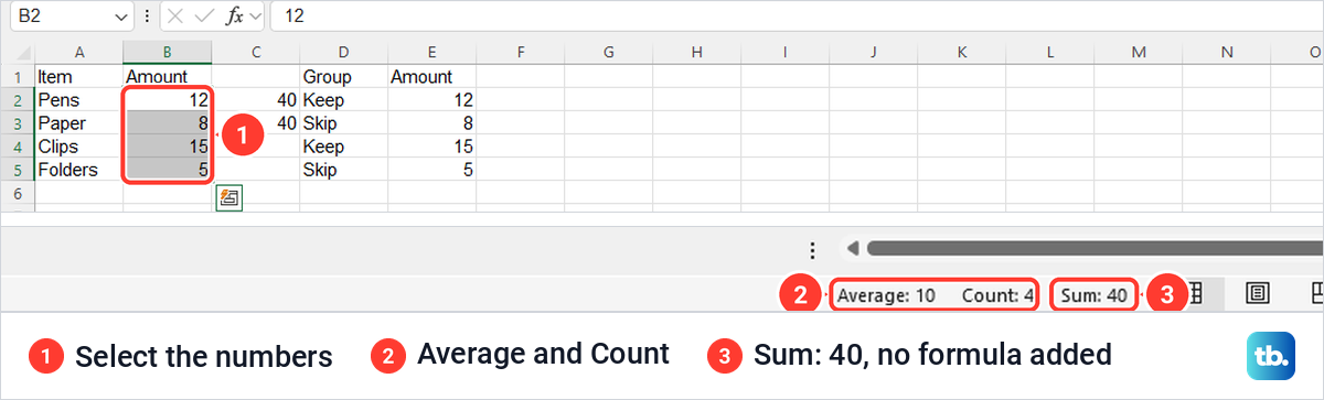
If Sum is missing, right-click the status bar to open Customize Status Bar and tick Sum. If the menu is taller than your window, scroll down inside it to reach Sum, which is ticked by default. The same menu also offers Numerical Count, Minimum and Maximum.
Build the formula with Insert Function
The Insert Function dialog helps if you do not remember a function's name. Click the empty cell, select the fx button beside the formula bar, type SUM under Search for a function and select Go. SUM came first in the list, with the description Adds all the numbers in a range of cells.
Select OK, then check the Number1 box before you go any further. In C5 on our sheet Excel had filled it with B5 alone, the cell to its left, and the dialog showed Formula result = 5.
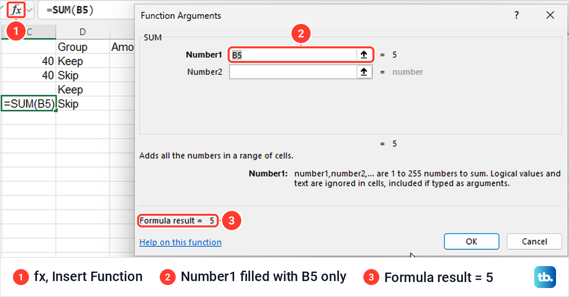
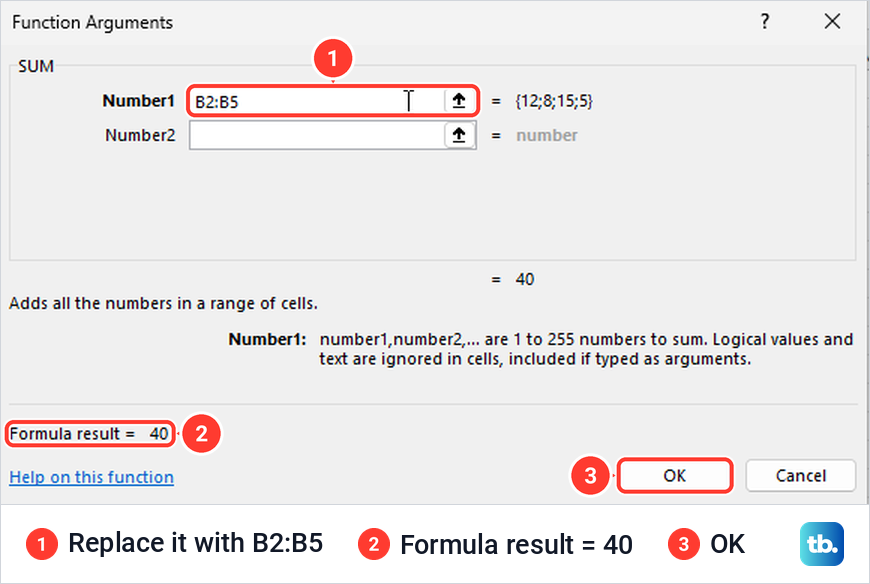
That pre-filled box is the trap in this method. Excel suggests cells next to the one you picked, and if you click OK without looking you get the wrong total with no warning. We replaced it with B2:B5, the result line changed to 40, and OK put 40 in C5.
Add a Total Row to an Excel table
An Excel table can keep its own total under the list. Select any cell in your data, choose Insert > Table, check the range, tick My table has headers only if the first row holds headings, then select OK. Our Group and Amount list in D1:E5 became a table named Table1.
Click inside the table, open the Table Design tab and tick Total Row. On our sheet a Total row appeared at once with 40 under Amount, already summed, and the formula bar showed =SUBTOTAL(109,[Amount]). Microsoft's help page says the cells are empty the first time you add a total row, so if yours is blank, select the cell, open its arrow and choose Sum.
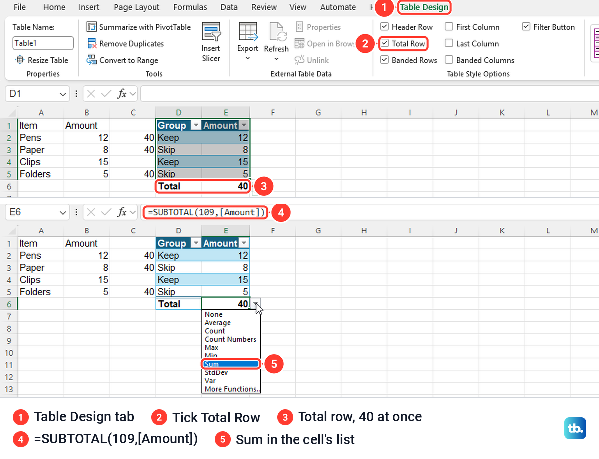
The arrow on each Total row cell lists None, Average, Count, Count Numbers, Max, Min, Sum, StdDev, Var and More Functions, so each column can have its own kind of total. For separate totals by category across a larger list, create a pivot table in Excel instead of adding many single-column totals.
Sum only the rows a filter shows
A plain SUM adds every cell in its range, hidden or not. That is usually what you want, but not when you filter a list and expect the total to match the screen. The table Total Row handles this for you, because the 109 in its SUBTOTAL formula tells Excel to leave filtered rows out.
We filtered our table's Group column to show only Keep. Rows 3 and 5 disappeared, the Total row changed from 40 to 27, and the formula stayed =SUBTOTAL(109,[Amount]). A filter hides whole worksheet rows, so anything beside the table in those rows disappears from view as well.
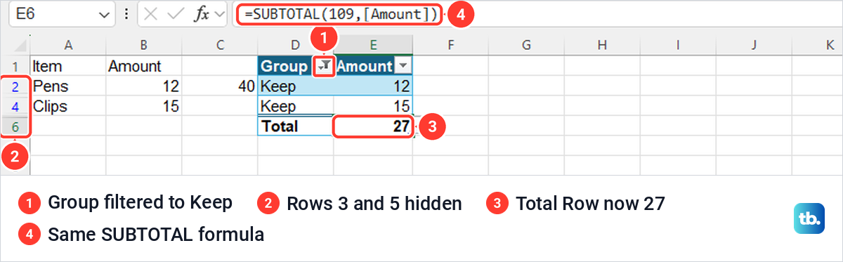
On an ordinary range, without a table, type the function yourself. With a filter hiding our Skip rows, =SUM(E2:E5) still showed 40 while =SUBTOTAL(109,E2:E5) showed 27. Put the formula in a row below the filtered list, because a filter hides whole rows and would hide a total that sits beside the data.
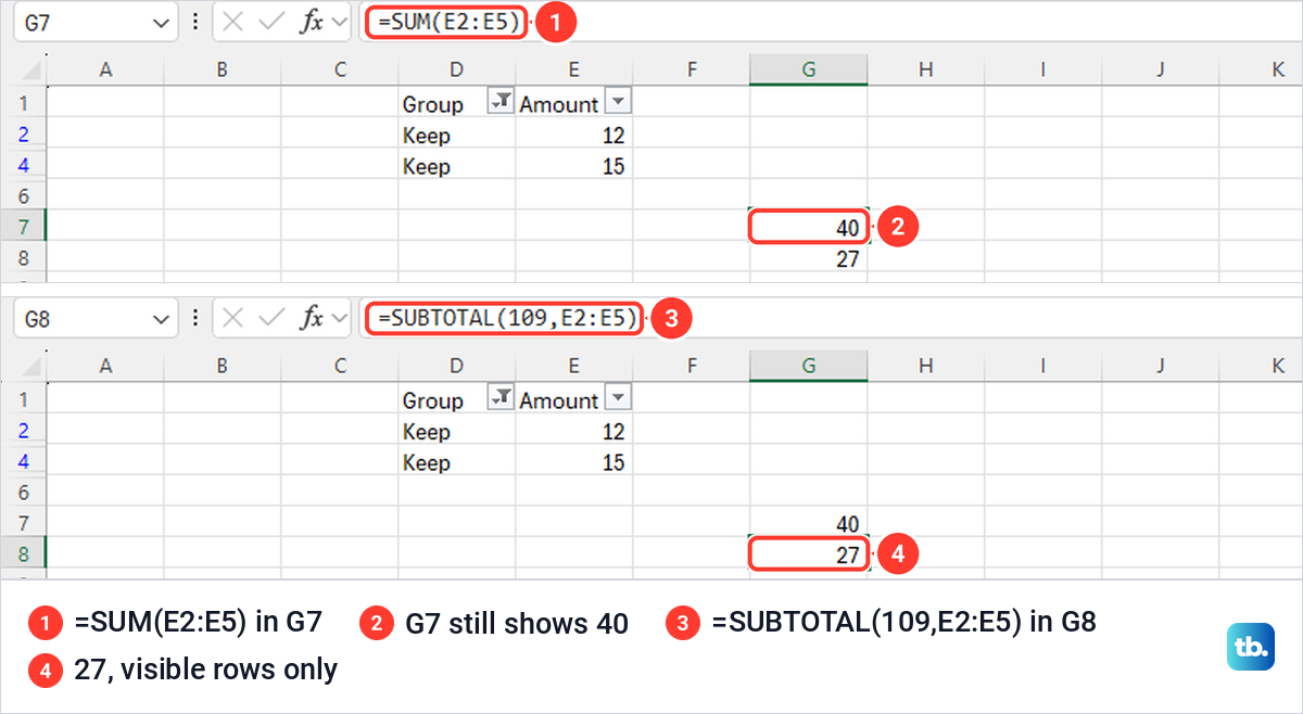
The function number decides what counts as hidden. Microsoft says 1 to 11 include manually hidden rows while 101 to 111 exclude them, and filtered-out cells are always excluded. So 9 and 109 both skip filtered rows, but if you hide rows in Excel by hand, only 109 leaves those amounts out.
If the filter arrows are missing or do nothing, fix an Excel filter that will not work first. Then filter the list again and check that the visible-row total changes with it.
Sum a column in Excel for the web
Excel for the web in Microsoft Edge sums a column the same way. In a new workbook holding the same four amounts, Home > AutoSum proposed =SUM(B2:B5) for B6 and the total was 40. Typed =SUM(B2:B5) and =SUBTOTAL(109,B2:B5) formulas gave 40 each, and the formula bar showed each one.
The Formulas tab has its own AutoSum button, and its arrow lists more than the desktop one. It starts like the desktop list, with Sum, Average, Count Numbers, Max and Min, and Sum shows its Alt + = shortcut. Below those, Excel for the web adds Add, Minus, Multiply and Divide. Choosing Sum proposed the same range and gave 40.
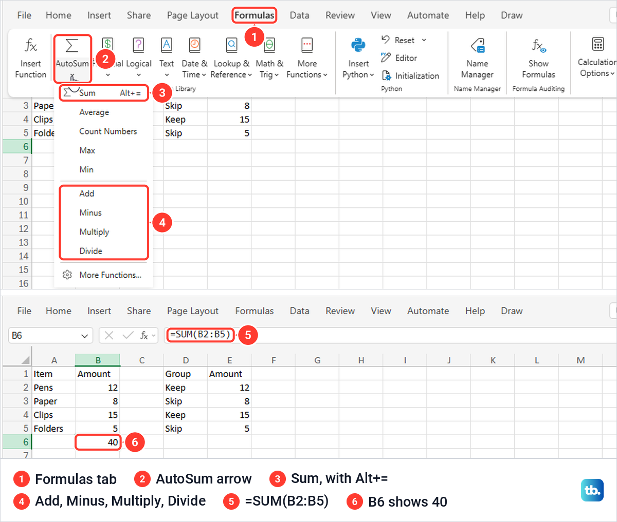
The status bar works much as it does on the desktop. Selecting B2:B5 showed Average: 10, Count: 4 and Sum: 40, and the arrow beside those values opened a Customize Status Bar panel with Average, Count and Sum ticked. Microsoft adds that in Excel for the web you can select a value such as Sum to copy it to the clipboard.
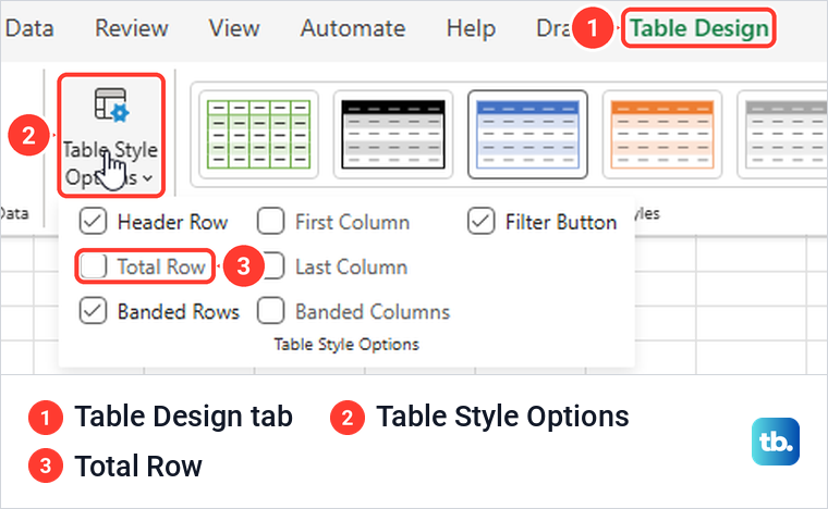
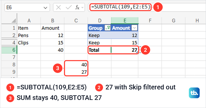
Tables differ in one place. After Insert > Table, the Total Row box sits inside a Table Style Options drop-down on the Table Design tab, which Microsoft's help page calls Style Options. Our web Total row showed 40, and after we chose Sum from its list the formula read =SUBTOTAL(109,E2:E5), with cell addresses instead of the column name.
Filtering Group to Keep changed that web total to 27. Because the filter hid whole rows, =SUBTOTAL(109,B2:B5) over the first list dropped to 27 as well, while =SUM(B2:B5) stayed at 40, the same split as on the desktop.
Fix an AutoSum range that stops too soon
When you use AutoSum below a column, it proposes the unbroken block of numbers directly above the cell. Microsoft puts it plainly: Excel selection stops at the first gap. On our sheet, with B4 left empty, AutoSum in B7 proposed =SUM(B5:B6), which would have added 15 and 5 and left out 12 and 8.
Fix it before you press Enter. While the dashed border is showing, drag over the whole column of numbers, B2:B6 in our case, and the formula changes to =SUM(B2:B6). Enter then gave 40, and the empty B4 did no harm.
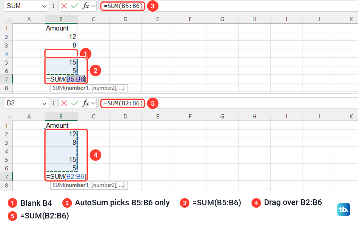
If the total is already in place, click it and read the formula bar. A range that starts lower than your first number, such as B5 instead of B2, is the giveaway, and typing the full range fixes it.
Fix numbers and formulas stored as text
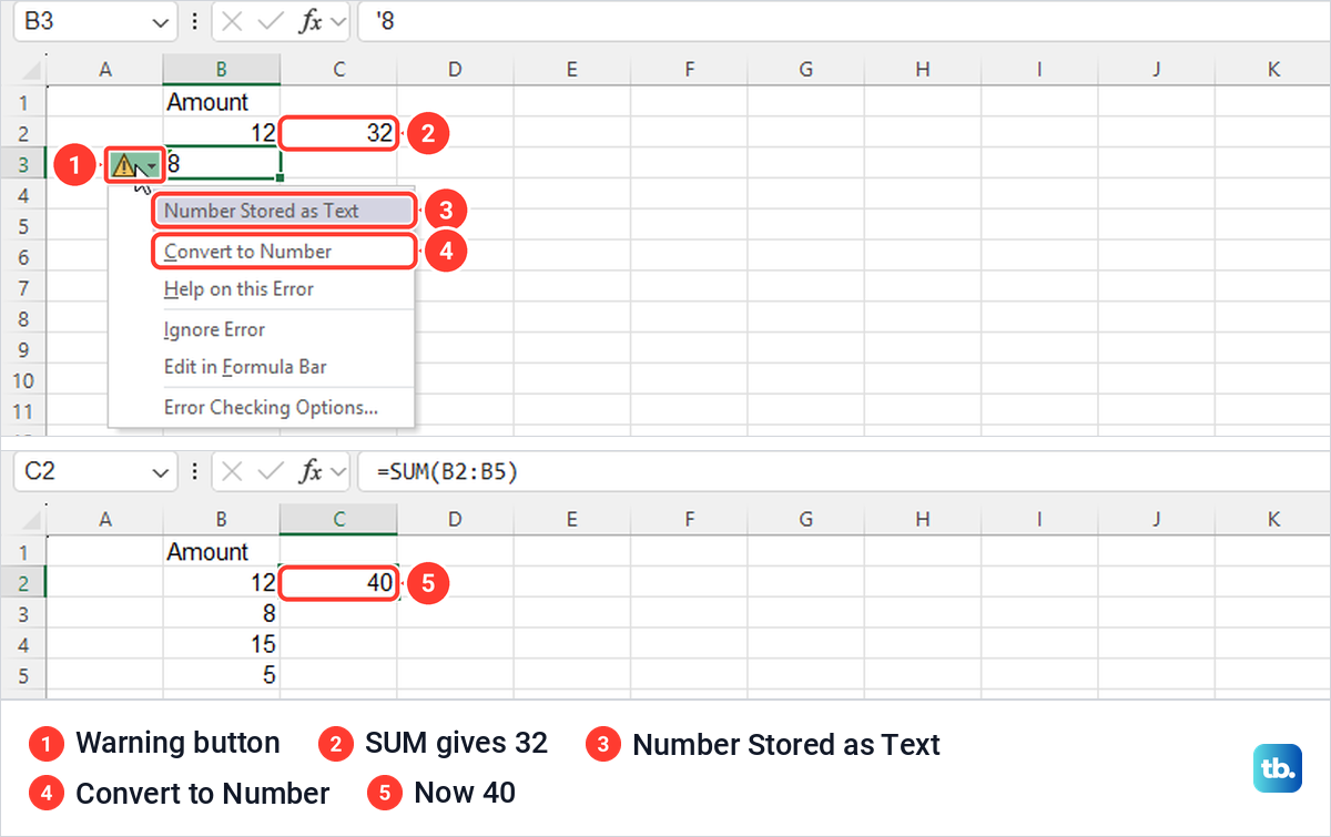
A number stored as text looks like a number, but SUM skips it. We typed the 8 in B3 as '8, and Excel marked the cell with a small green triangle while =SUM(B2:B5) returned 32 instead of 40. Amounts that arrive after you convert a PDF to Excel or paste from another app are worth this check before you rely on a total.
Select the cell with the triangle, then the warning button that appears beside it. The menu is headed Number Stored as Text, and Convert to Number fixed our total, which went from 32 to 40.
A formula can be stuck as text too. In a cell formatted as Text, our =SUM(B2:B3) showed as the formula itself instead of a result. Changing the format to General on the Home tab did not fix it by itself, but pressing F2 and then Enter did, and the cell showed 20.
Microsoft gives the same order, General first and then F2 and Enter. If the formula still shows as text, here is how to fix an Excel formula showing as text for the other causes. If the range and the cell types are right but the total still looks wrong, work through how to fix a SUM formula that is not working.
Clear a circular reference or a protected sheet
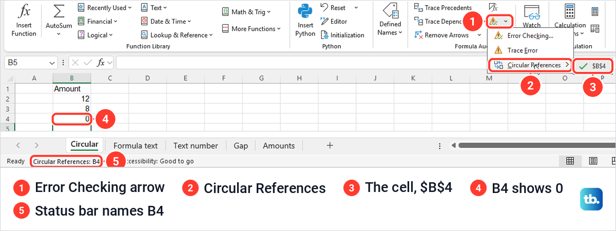
A whole-column SUM inside its own column refers to its own cell. When we typed =SUM(B:B) in B4, Excel warned that there are one or more circular references where a formula refers to its own cell. After OK, the cell showed 0.
To find the cell, open the Formulas tab, select the arrow beside Error Checking, a warning-triangle icon in the Formula Auditing group, and point at Circular References. Ours listed $B$4, and the status bar at the bottom left read Circular References: B4. Changing B4 to =SUM(B2:B3) showed 20, and the status bar message went away.
A protected sheet can stop you entering a total, because Microsoft says protection prevents changes to locked cells. On ours, Excel said The cell or chart you're trying to change is on a protected sheet, and the button on the Review tab read Unprotect Sheet. After we selected it, the same =SUM(B2:B3) went in and showed 20.
If the sheet has a password, Excel asks for it when you select Unprotect Sheet, and Microsoft warns that it cannot retrieve a forgotten password. Before you change protection, see how to lock cells in Excel and what protection covers. If an amount changes but the total does not, fix Excel formulas that stop calculating, because a workbook in manual calculation mode keeps old results.
How we tested this guide
We tested this in Excel for Microsoft 365 on Windows 11, version 25H2, and in Excel for the web in Microsoft Edge, summing a column of made-up amounts.
Frequently Asked Questions
What is the fastest way to sum a column in Excel?
Click the empty cell under the numbers and press Alt + =, or select Home > AutoSum. Check the range Excel highlights, then press Enter.
How do I sum a whole column as I add new numbers?
Put =SUM(B:B) in another column and keep any total row out of column B, or it is counted again. On our sheet that mistake turned 40 into 80.
Why does AutoSum leave out numbers above a blank cell?
AutoSum stops at the first gap above the cell. Drag over the full range before you press Enter, or type it yourself, such as =SUM(B2:B6).
Can I see the total without adding a formula?
Yes. Select the numbers and read Sum on the status bar at the bottom of the window, which is on by default.
How do I sum only the visible rows after filtering?
Use a table Total Row, or =SUBTOTAL(109,E2:E5) in a row below the filtered list. Plain SUM keeps adding hidden rows, which is why ours stayed at 40 while SUBTOTAL showed 27.
Why is my SUM total zero or too low?
Check that the formula covers every number, and look for green triangles that mark numbers stored as text. Convert to Number fixed a total of 32 that should have been 40 on our sheet, and a circular reference showed 0.
Can the total go in the same column as the numbers?
Yes, as long as it uses a bounded range such as =SUM(B2:B5) below the last number. A whole-column =SUM(B:B) inside column B is a circular reference.
How do I sum a column in Excel on a Mac or an Android phone?
Microsoft's Mac steps are to click the first empty cell below the numbers, select AutoSum on the Formulas tab and press Return, and its Mac shortcut is Shift + Command + T. On Android, Microsoft says to tap the first empty cell after the numbers, tap AutoSum, tap Sum and then tap the check mark.