
To hide a column in Excel, right-click the column letter at the top of the sheet and choose Hide. To hide several columns, drag across their letters first, then right-click any of them. The column disappears from view, but its data stays in the workbook and formulas keep using it.
To bring a column back, select the letters on both sides of the gap, right-click and choose Unhide. A double line between two letters marks the place where a column is hidden.
The short version
- One column: right-click the column letter and choose Hide.
- Several columns: drag across the letters, or hold Ctrl as you select separate ones, then choose Hide.
- Keyboard on Windows: Ctrl + Spacebar selects the column and Ctrl + 0 hides it.
- Spot a hidden column: the letters skip one, and a double line marks the gap.
- One-click toggle: group the columns from Data > Outline > Group and use the minus button.
Ways to hide columns in Excel at a glance
| Method | How to do it | What you get |
|---|---|---|
| Right-click menu | Select the column letter, right-click it and choose Hide | The column vanishes and the letters skip one |
| Home tab | Home > Format > Hide & Unhide > Hide Columns | The same result from the ribbon |
| Ctrl + 0 | Select the column with Ctrl + Spacebar first | The fastest route in Excel for Windows |
| Column width 0 | Home > Format > Column Width, type 0 and select OK | The column is hidden, and a positive width shows it again |
| Group | Data > Outline > Group, then the minus button | The columns collapse behind a plus button that opens them again |
| Excel for the web | Right-click the column letter and choose the Hide Column item | The same result in a browser, where the menu names the column |
| Excel for Mac | Select the column letters, right-click and choose Hide | The same steps Microsoft gives for Windows |
The first four methods hide the column outright, and its data stays where it was. A group works differently, because it adds its own plus and minus buttons above the letters, which suits columns you open and close often.
Hide a column with a right click
Click the letter at the top of the column you want to hide, so the whole column is selected. Right-click the letter and choose Hide near the bottom of the menu. On our sheet that menu ended with Format Cells, Column Width, Hide and Unhide.
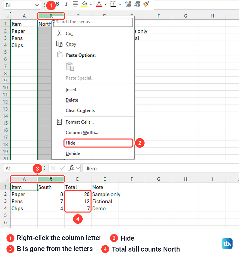
Column B, North, disappeared at once, and the letters along the top went from A straight to C. Microsoft describes a double line between two column letters as the sign that a column is hidden there. Nothing was deleted, and our Total column, which adds North and South with SUM, still showed 20, 12 and 7.
That result is for SUM, the formula on our sheet, and other kinds of formula are worth checking after you hide a column. If you are still building the total itself, our guide to sum a column in Excel covers SUM and AutoSum.
Rows work the same way from the numbers down the left edge. If those are what you want out of view, follow the steps to hide rows in Excel instead.
Hide several columns at once
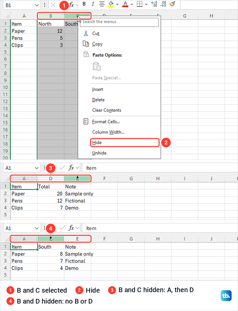
For columns that sit next to each other, click the first letter and drag across to the last one. We dragged across B and C, right-clicked the highlighted letters and chose Hide, which left A, D and E on screen in one step.
Columns that are apart can be hidden in one go too. Once B and D were both selected on our sheet, Hide removed both and left A, C and E. To select columns like that, Microsoft says to press and hold Ctrl as you select each additional column.
Hidden columns come back together too. Selecting A through E and choosing Unhide restored every column on our sheet, with all of its numbers.
Hide columns from the Home tab
The ribbon has the same command, with Hide Rows and Hide Sheet beside it. Select the column, open Home > Format in the Cells group, point to Hide & Unhide under Visibility and choose Hide Columns.
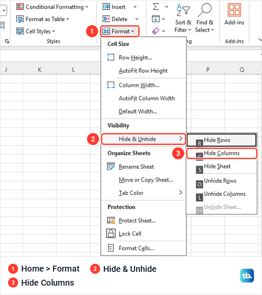
On our sheet Hide Columns removed column C, and Unhide Columns in the same submenu brought it back. The Format menu also holds Column Width under Cell Size, which is another way to hide a column, covered below.
Use the Excel hide column shortcut
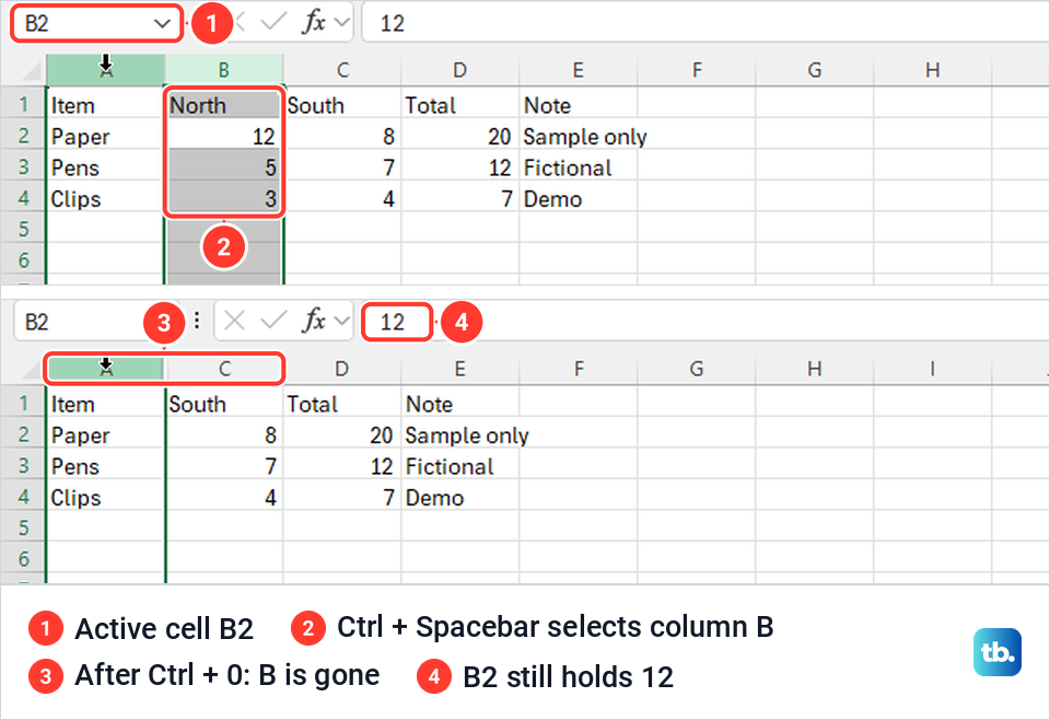
In Excel for Windows, the keyboard is the fastest route. Click any cell in the column, press Ctrl + Spacebar to select the whole column, then press Ctrl + 0. Microsoft lists both in its Excel shortcut table, and both worked on our PC.
From cell B2, Ctrl + Spacebar highlighted all of column B, and Ctrl + 0 hid it. The Name Box still read B2 and the formula bar still showed 12, so the hidden cell kept its value and stayed selected.
Microsoft lists Ctrl + 0 for Excel for the web as well, but in our Edge session it did not hide the column. If the shortcut does nothing for you, use the right-click menu instead. For other selection and navigation keys, see our Excel keyboard shortcuts guide.
Hide a column by setting its width to zero
A column with a width of 0 is a hidden column. Microsoft's column size table lists 0 as hidden, and that is exactly what happened on our sheet.
Select the column, then go to Home > Format > Column Width, or right-click the column letter and choose Column Width. Type 0 and select OK. Our Note column, E, vanished and the letters jumped from D to F.
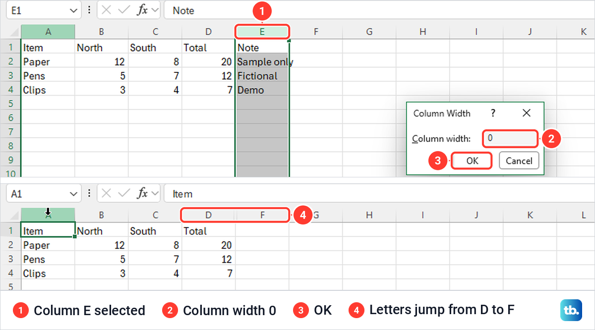
Check the old width before you change it, so you can set it back. Ours read 8.38, close to the 8.43 that Microsoft's size table lists as the standard width, so the number in your workbook may differ. To show the column again, type E1 in the Name Box beside the formula bar and press Enter, then open Column Width, type a width above zero and select OK.
Typing 8.38 brought our column E back. Any width above zero shows the column again, so pick the one that suits your data.
Group columns so they collapse with one click
If you hide and show the same columns often, a group is quicker than Hide and Unhide. Select the detail columns, leaving out the total you want to keep in view. Then on the Data tab, select Group in the Outline group and choose Group again from its short list. In our window the Outline group had shrunk to a single Outline button, so we opened that first.
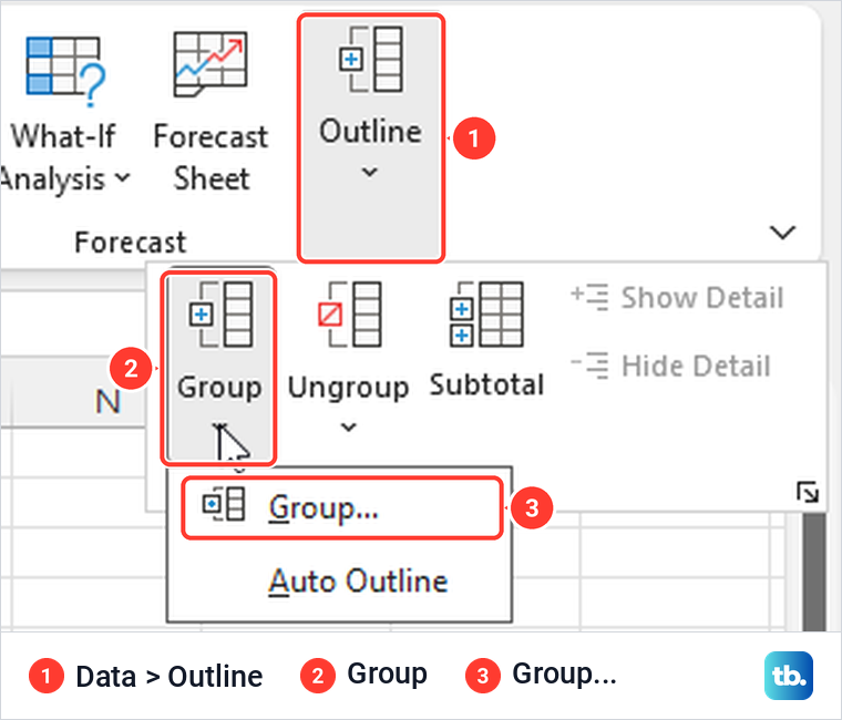
We selected B and C, North and South, and grouped them. Excel added a bar above the letters with a minus button over column D, and level buttons 1 and 2 at the left. Because whole columns were selected, no dialog asked about rows or columns.
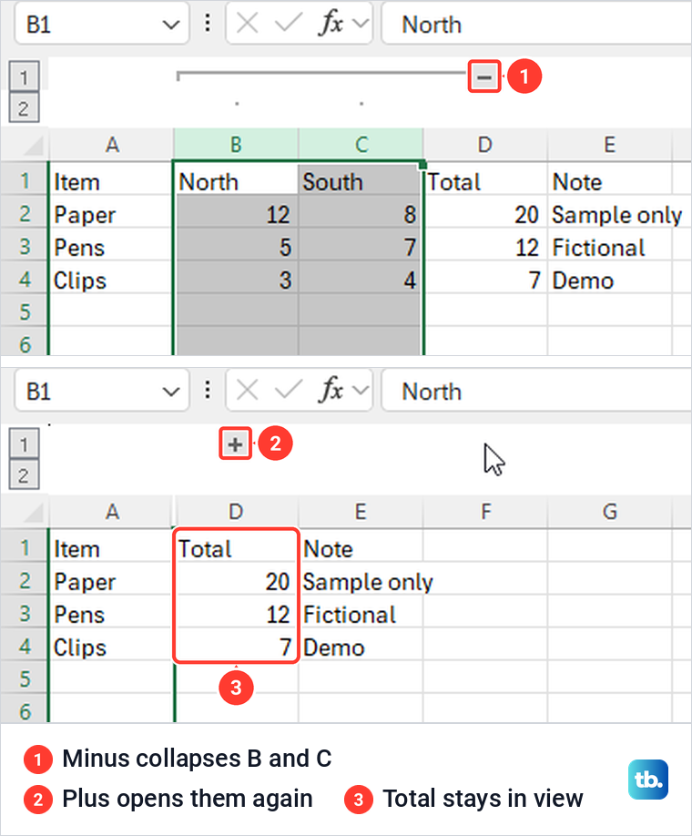
Selecting the minus button collapsed B and C while the Total column stayed on screen, and the minus turned into a plus. Selecting the plus opened both columns again. Microsoft also lists Alt + Shift + - to hide a group's detail and Alt + Shift + = to show it.
A group suits columns other people may need, because the plus button tells them there is more to see. To remove it, select the columns and choose Data > Outline > Ungroup.
Hide columns in Excel for the web
The browser version uses the same right-click route, with clearer labels. Make sure the workbook is in Editing mode, right-click the column letter and choose the Hide item, which names the column. On our sheet it said Hide Column B, and with A to C selected it said Hide Columns A - C.
After Hide Column B, the letters ran A, C, D, E with a double line between A and C. Selecting A to C again offered Unhide Columns, which brought North back. If you have not opened a workbook in a browser before, our Excel for beginners guide shows where to find Excel for the web.
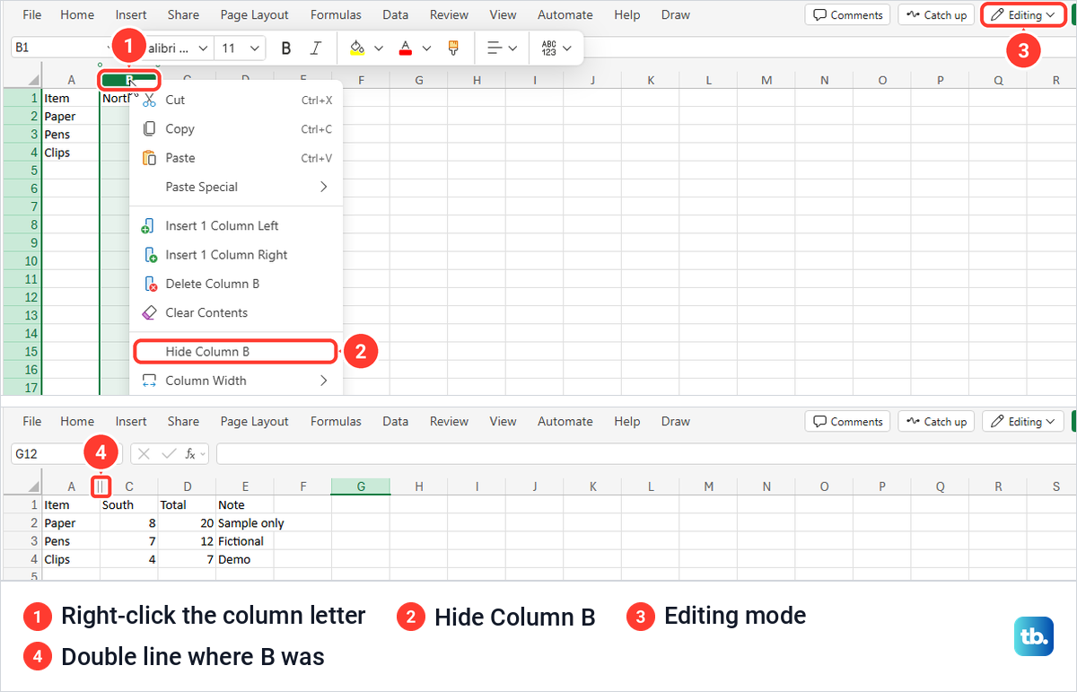
Microsoft says that when formatting and other changes do nothing in a browser workbook, you are probably in read-only view, and the fix is to select Editing. The mode button sits at the top right, and ours read Editing when we hid column B.
The keyboard shortcut is where our web session differed. With column C selected in Edge, Ctrl + 0 left it on screen. Nothing on the sheet changed.
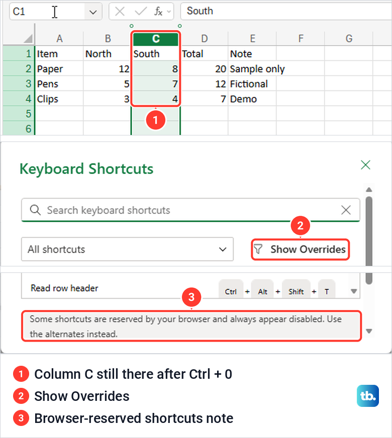
The web app's own Help > Keyboard Shortcuts dialog carries a note that some shortcuts are reserved by your browser and always appear disabled, and it says to use the alternates instead. It also has a Show Overrides filter. For hiding columns, the alternate is the right-click menu, which worked on our sheet.
Columns can be grouped in the browser too. Microsoft's steps are to select the columns, go to Data > Outline > Group > Group and choose Columns, then use the plus and minus buttons as on the desktop.
Hide columns in Excel for Mac
Microsoft's hide and show instructions cover Excel for Mac as well as Windows. Select one or more column letters, then select and hold, or right-click, the selection and choose Hide. To show them again, select the columns on both sides and choose Unhide the same way.
Why Hide is missing or greyed out
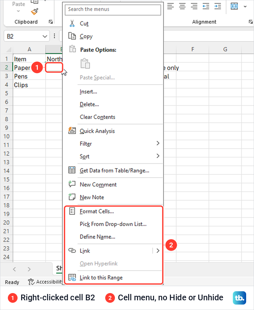
In the right-click menu, Hide appears when you right-click a column letter, not a cell. Right-clicking a cell opens a longer menu, and the one for cell B2 on our sheet had Quick Analysis, Filter, Sort and Format Cells but no Hide or Unhide. Right-clicking the B letter above it showed Hide straight away.
When Hide is there but greyed out, check whether the sheet is protected, because a protected sheet can grey out Hide when Format columns is not allowed. We protected our sheet from Review > Protect Sheet with the options as they opened, and Format columns was unticked by default. After that, Column Width, Hide and Unhide were greyed out in the column menu, and Excel showed no message at all.
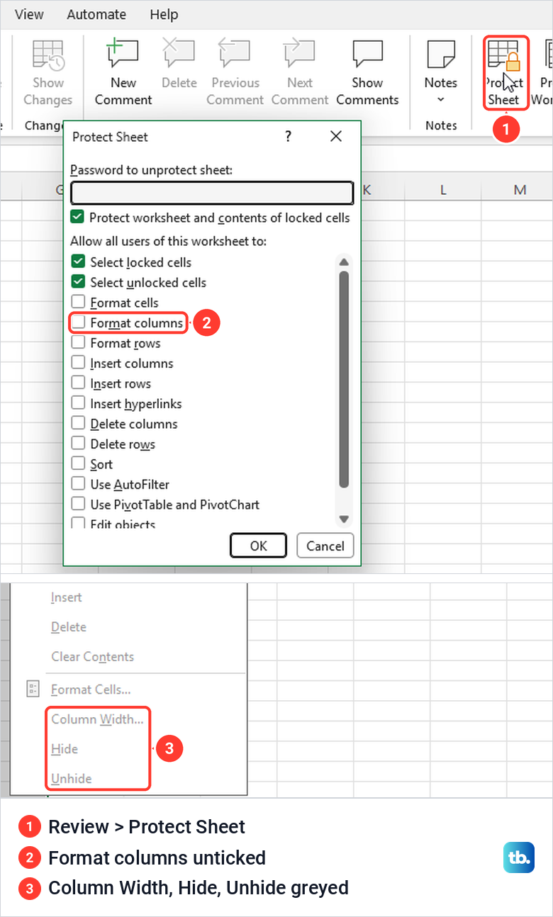
Microsoft's protection table says the Format columns option covers changing column width and hiding columns. So either whoever protects the sheet ticks Format columns, or someone with the right to change it removes the protection. When Review shows Unprotect Sheet and you have authority to change it, unprotect an Excel worksheet first, and column C then hid and unhid normally on our sheet.
What hiding a column does not do
Hiding is about what you see, not who can see it. Unhide sits on the same menu as Hide, so anyone working in the file can bring the column back, and Microsoft says even worksheet protection isn't intended as a security feature. If someone must not be able to open the workbook at all, password protect the Excel file rather than hiding a column.
To stop people changing values while leaving them visible, lock cells in Excel and protect the sheet with the permissions you want. To keep a column on screen while you scroll sideways, freeze cells in Excel rather than hiding the columns in between.
For printing, Microsoft's Excel for the web help says hidden rows and columns won't be printed. To include them, unhide them before you print.
In a workbook other people use, hiding a column changes their view too unless you work in a Sheet View. Microsoft says a Sheet View lets you hide columns without changing the view for others, but you must enter the Sheet View first, and a column hidden in the Default view stays hidden in every Sheet View. Sheet Views only work in files stored in OneDrive or SharePoint.
For a file kept on your PC, make a copy of the Excel file and delete the columns the reader must not have from that copy, because hidden data travels with the file. Hide columns in the copy only to tidy what is left.
Bring a hidden column back
To show a hidden column, select the letters on both sides, right-click and choose Unhide. Column A is the awkward one, and on our PC Unhide on the B letter alone left A hidden, while typing A1 in the Name Box and choosing Home > Format > Hide & Unhide > Unhide Columns worked. Our guide to bring back hidden columns in Excel covers the other routes, including several gaps at once.
How we tested this guide
We tested this in Excel for Microsoft 365 on Windows 11, version 25H2, and Excel for the web in Microsoft Edge, hiding columns on a made-up sales sheet.
Frequently Asked Questions
Does hiding a column delete its data?
No. The values stay in their cells and formulas keep using them. On our sheet the North figures came back as 12, 5 and 3 after Unhide, and the totals counted them the whole time.
How do I hide multiple columns at once?
Drag across the letters of columns that sit together, or hold Ctrl as you select separate columns, as Microsoft describes. Then right-click any selected letter and choose Hide.
What is the shortcut to hide a column in Excel?
In Excel for Windows, press Ctrl + Spacebar to select the column, then Ctrl + 0 to hide it. Microsoft lists Ctrl + 0 for Excel for the web too, but it did not hide the column on our sheet in Edge, so use the right-click menu when the shortcut does nothing.
Why is Hide missing when I right-click?
You probably right-clicked a cell rather than the column letter, and the cell menu has no Hide. If Hide is there but greyed out, the sheet may be protected without the Format columns permission.
Can I make columns collapse with one click?
Yes. Select the columns and choose Data > Outline > Group, and Excel adds a minus button that collapses them and a plus button that brings them back.
Can other people see a hidden column?
Assume they can, because hiding is not a privacy setting. Unhide sits on the same menu as Hide, so keep data someone must not read out of the file you share.