
To round in Excel, select the cells and click Decrease Decimal in the Number group on the Home tab if the numbers only need to look rounded. If later formulas should use the rounded value, type =ROUND(A2,2) in another cell instead, where 2 is the number of decimal places to keep. Formatting leaves the full number in the formula bar and in every calculation, while ROUND returns a new, rounded value in its own cell.
Two results are worth knowing before you start. A new ROUND cell can pick up the number format of the cell it points at and hide its own result, and MROUND, the function Microsoft's own rounding guide uses for counting crates, came up short on our sheet.
The short version
- Change how it looks: select the cells and click Home > Decrease Decimal, or press Ctrl + 1 and set Decimal places.
- Calculate with a rounded value: in another cell, use the Excel ROUND function,
=ROUND(A2,2)for two decimals,=ROUND(A2,0)for a whole number or=ROUND(A2,-1)for the nearest ten. - Always up or down: ROUNDUP moves away from zero and ROUNDDOWN toward zero, which matters for negative numbers.
- To a multiple: MROUND finds the nearest one, while CEILING.MATH and FLOOR.MATH go up or down for positive numbers.
- Looks wrong? Check the result cell's format and the column width first, and leave Set precision as displayed off unless you mean to change stored data for good.
Choose whether to round the look or the value
Excel rounds a number in two different ways, and picking the wrong one causes most rounding confusion. Number formatting changes only what the cell shows. Microsoft's help says a formatted number appears rounded while the entire number stays in the formula bar and is still used in calculations.
A rounding function returns a new number instead. The original cell keeps its full value, and the formula cell holds the rounded result that later formulas pick up when they point at it. Use formatting for reports and printouts, and a function when totals, exports or comparisons must use the rounded figure.
Totals are where the difference shows. A sum adds the stored values, so a column of prices that each look rounded can add up to a total a cent away from what the visible figures suggest. To fix it, type =ROUND(A2,2) in the first row of a spare column, drag the fill handle (the small square at the cell's bottom-right corner) down to the last row, then sum a column in Excel from those results.
| What you need | Use | On our sheet |
|---|---|---|
| Fewer decimals on screen | Home > Decrease Decimal | 23.7825 showed as 23.78 |
| An exact number of decimals on screen | Ctrl + 1, Number, Decimal places | 823.7825 showed as 824 at 0 places |
| A rounded value to calculate with | =ROUND(A2,2) | 23.7825 gave 23.78 |
| A whole number or the nearest ten | =ROUND(A3,0) or =ROUND(A3,-1) | 823.7825 gave 824 or 820 |
| Always away from zero | =ROUNDUP(A4,2) | 3.14159 gave 3.15 |
| Always toward zero | =ROUNDDOWN(A4,2) | 3.14159 gave 3.14 |
| The nearest multiple | =MROUND(A9,5) | 7.5 gave 10 |
| The next multiple up or down | =CEILING.MATH(A9,5) or =FLOOR.MATH(A9,5) | 7.5 gave 10 or 5 |
| No decimals, no rounding | =TRUNC(A7) | -12.6 gave -12 |
| Every number stored as shown | File > Options > Advanced > Set precision as displayed | 1.2345 became 1.23 for good |
Only the last row changes the original numbers. Every formula row puts its result in a new cell and leaves the source cell exactly as it was.
Show fewer decimal places with Decrease Decimal
Select the cells you want to change. On the Home tab, find the Number group and click Decrease Decimal, the right-hand button of the pair beside the Comma Style button. Each click hides one more decimal place, and its neighbour, Increase Decimal, shows one more.
On our sheet, A2 held 23.7825. The first click showed 23.783 and the second 23.78, and the Number Format box above the buttons changed from General to Number. The formula bar still read 23.7825 after both clicks, so any formula that uses A2 still sees all four decimal places.
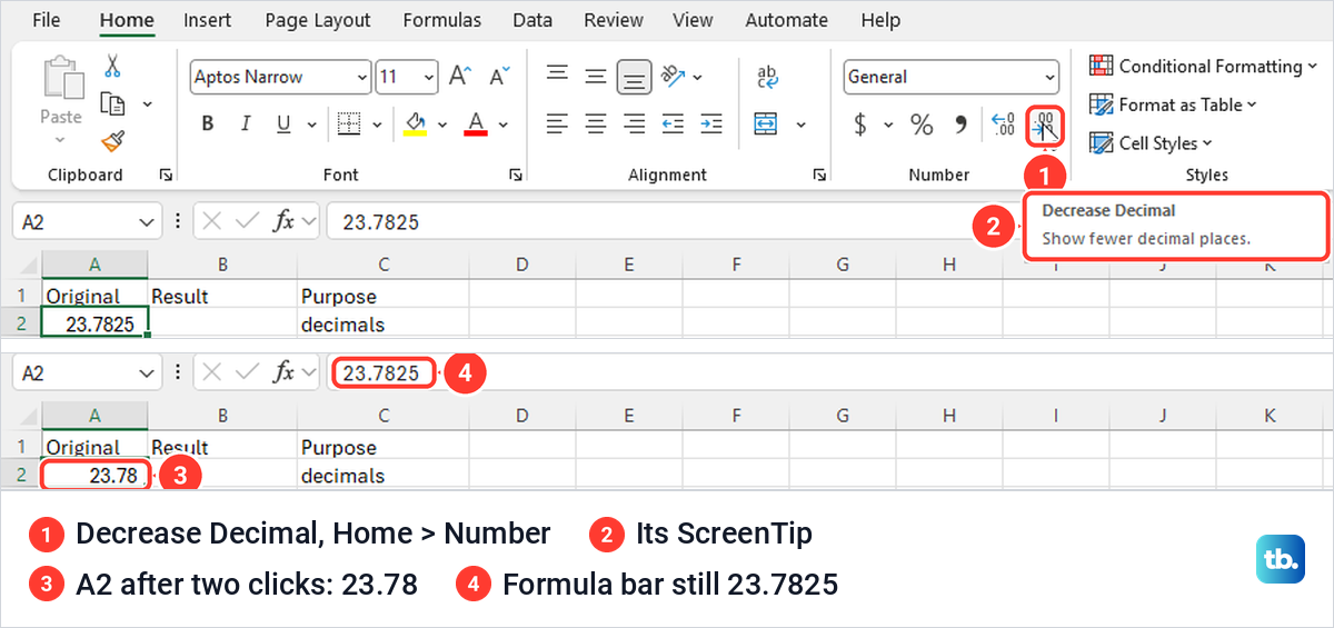
One click of Increase Decimal brought back 23.783, which shows the digits were only hidden. Microsoft's steps start by selecting the cells you want to format, so a whole column of prices can be set in one go.
Set an exact number of decimal places in Format Cells
The buttons work by counting clicks, which gets fiddly when a column mixes numbers of different lengths. Format Cells sets an exact number of places instead. Select the cells, open the Number Format list on the Home tab and choose More Number Formats at the bottom.
In the Format Cells box, pick Number under Category, type the places you want in Decimal places and click OK. Excel filled in 2 for our General cell, and the Sample line previews the result before you commit. With 0 places, our 823.7825 showed as 824, and the formula bar kept 823.7825.
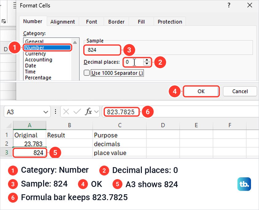
Two faster ways open the same box. Press Ctrl + 1, or right-click the cell and choose Format Cells. We used both, and two decimal places made 3.14159 show as 3.14 and -3.14159 as -3.14, with the full values still in the formula bar. Ctrl + 1 is one of the Excel keyboard shortcuts worth learning if you format numbers often.
Round a number with the ROUND function
When the rounded figure has to be the real value, use ROUND. Its form is =ROUND(number, num_digits), where number is the value or cell to round and num_digits says how many decimal places to keep. Excel shows that pattern in a ScreenTip under the cell as soon as you type =ROUND(.
Click an empty cell next to your data, type =ROUND(A2,2) and press Enter. On our sheet it returned 23.78 for 23.7825. A2 keeps its original value and the new cell holds the rounded one, so point later formulas at the new cell.
The first part can also be a whole calculation, as in =ROUND(B2*C2,2), which rounds a product in one step after you multiply values in Excel. The same works when you subtract one cell from another and need the difference to two decimals. If the result is a rate, calculate the percentage in Excel first and keep two more digits than the percentage should show, because 12.34% is stored as 0.1234.
Use the Function Arguments box instead of typing
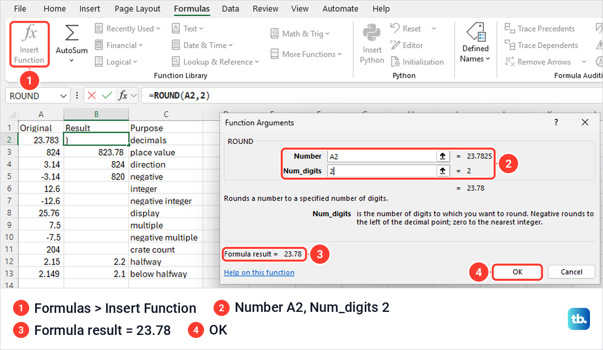
If you prefer boxes to typing, click the empty cell and select Formulas > Insert Function. Type ROUND in the search box and select Go. Excel listed ROUND first, then ROUNDDOWN, ROUNDUP, MROUND, CEILING and CEILING.MATH, with the line Rounds a number to a specified number of digits. Pressing Shift + F3 opened the same Insert Function box on our PC.
Select ROUND and click OK to open Function Arguments. Fill in Number (A2 in our case) and Num_digits (2), and the box shows Formula result = 23.78 before anything reaches the sheet. Click OK to place the formula.
Check the format of the result cell
One thing can make a correct ROUND look wrong. When we clicked OK, B2 showed 23.780, not 23.78, even though the dialog had shown 23.78. B2 had taken on the three-decimal format we gave A2 earlier with the decimal buttons, so the value was right and only the display was off.
It was more confusing in B3. There, =ROUND(A3,2) showed 824 instead of 823.78, because A3 had been set to zero decimal places and the new formula cell picked up the same Number format. Selecting B3 and pressing Ctrl + Shift + ~ to apply the General format showed 823.78 at once.
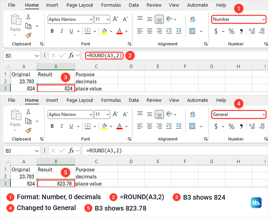
So if a ROUND result shows too few or too many digits, select the result cell and look at the Number Format box on the Home tab. Set it to General, or to Number with the places you want. The formula bar shows the formula itself in a formula cell, so the format box is the thing to check here.
Round to a whole number, tens or hundreds
The second part of ROUND decides where the rounding happens. A positive number keeps that many decimal places, 0 rounds to the nearest whole number, and a negative number rounds to the left of the decimal point, so -1 gives tens and -2 gives hundreds. The Function Arguments box spells it out too, saying negative rounds to the left of the decimal point and zero to the nearest integer.
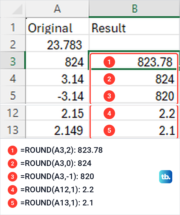
On our sheet, 823.7825 in A3 became 823.78 with =ROUND(A3,2), 824 with =ROUND(A3,0) and 820 with =ROUND(A3,-1). Halfway values went up, so =ROUND(A12,1) turned 2.15 into 2.2, while 2.149 in A13 became 2.1. A negative half moves away from zero, and =ROUND(-1.475,2) returned -1.48.
Round up or round down in Excel
ROUNDUP and ROUNDDOWN take the same two parts as ROUND but ignore the halfway rule. Microsoft describes ROUNDUP as rounding away from zero and ROUNDDOWN as rounding toward zero. For positive numbers that means up and down.
On our sheet, =ROUNDUP(A4,2) turned 3.14159 into 3.15 and =ROUNDDOWN(A4,2) turned it into 3.14. For -3.14159, =ROUNDUP(A5,1) returned -3.2 and =ROUNDDOWN(A5,1) returned -3.1. So with a negative number, ROUNDUP gives the smaller number and ROUNDDOWN the larger one.
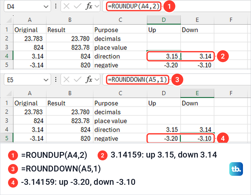
Our cells showed -3.20 and -3.10 with a trailing zero, because the new cells again copied the two-decimal format of A5. To round up in Excel to a whole number, use 0 digits. In our Excel for the web workbook, where A3 held 12.6, =ROUNDUP(A3,0) returned 13.
If a negative number should move toward zero instead, use ROUNDDOWN. Microsoft says CEILING.MATH rounds negative numbers toward zero by default and FLOOR.MATH rounds them away from zero, and each has a mode setting that reverses that.
Round to the nearest 5, 10 or any multiple
MROUND rounds to the nearest multiple of any number you choose, such as 5 for prices that end in 0 or 5. For positive numbers, CEILING.MATH always goes up to the next multiple and FLOOR.MATH always goes down. All three take the number first and the multiple second.
With 7.5 in A9 and a multiple of 5, =MROUND(A9,5) returned 10, =CEILING.MATH(A9,5) returned 10 and =FLOOR.MATH(A9,5) returned 5. MROUND went up here because 7.5 sits exactly halfway, and Microsoft says MROUND rounds away from zero when the remainder is at least half the multiple.
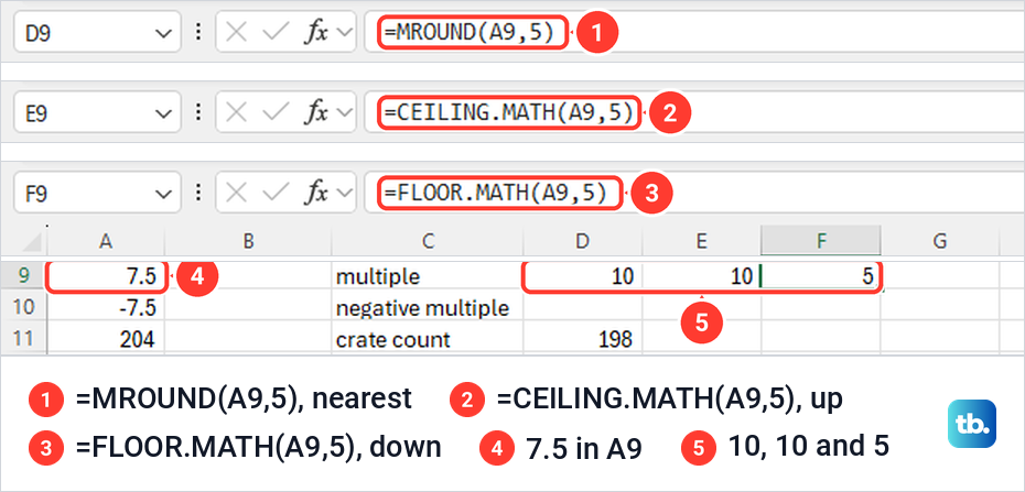
Choose by what must not happen. Use MROUND when the nearest multiple is fine, CEILING.MATH when you must never come in under the value, and FLOOR.MATH when you must never go over it. For the nearest ten, =ROUND(A2,-1) does the same job as MROUND with 10.
Do not use MROUND to count crates or boxes
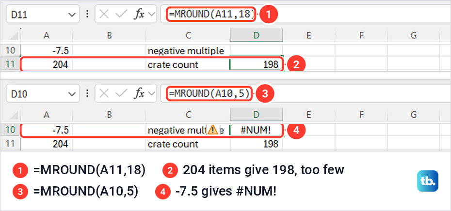
Microsoft's own rounding guide uses MROUND for a shipment of 204 items in crates of 18 and says the answer is 12 crates. We typed that case, and =MROUND(A11,18) returned 198. That is 11 full crates, six items short of the shipment, because MROUND rounds to the nearest multiple and 204 is closer to 198 than to 216.
When a quantity must be fully covered, round up instead. =CEILING.MATH(A11,18) rounds 204 up to the next multiple of 18, and =ROUNDUP(A11/18,0) gives the number of crates rather than the number of items. Both rely on the upward direction Microsoft documents for those two functions.
Fix #NUM! from MROUND
MROUND needs the number and the multiple to have the same sign. With -7.5 in A10, =MROUND(A10,5) showed #NUM!, and changing it to =MROUND(A10,-5) returned -10. Microsoft's MROUND page gives the same rule.
Remove decimals with INT or TRUNC
Sometimes you want the decimals gone rather than rounded. TRUNC cuts off the fraction, while INT rounds down to the next lower whole number. Microsoft explains the difference the same way, and it only shows with negative numbers.
For -12.6 in A7, =INT(A7) returned -13 and =TRUNC(A7) returned -12. TRUNC also takes a second part like ROUND, so =TRUNC(A2,2) keeps two decimal places and drops the rest without rounding.
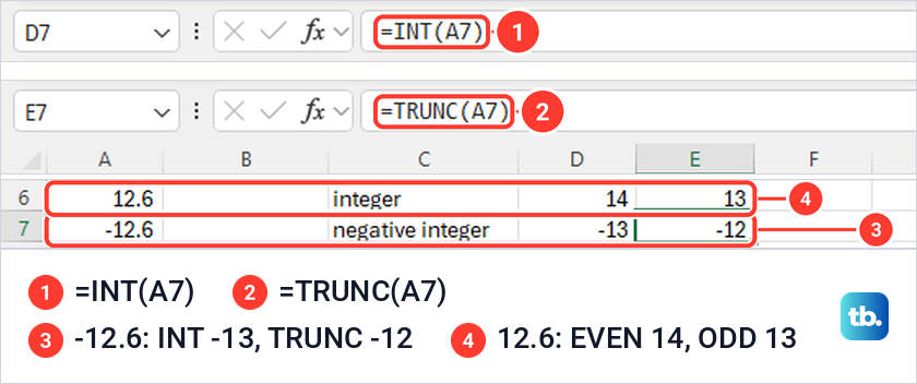
EVEN and ODD round away from zero to the next even or odd whole number. Our 12.6 became 14 with =EVEN(A6) and 13 with =ODD(A6). They are handy when items have to come in pairs.
Round numbers in Excel for the web
Excel for the web has the same tools on its Home tab. In Microsoft Edge, the two decimal buttons in the Number group sat in the opposite order to the desktop app. The left one was Decrease Decimal and the right one Increase Decimal, so hover over a button to read its ScreenTip before you click.
As on the desktop, our 23.7825 showed as 23.78 while the formula bar kept 23.7825. The Number Format list offers General, Number, Currency, Percentage and the rest, with More Number Formats at the bottom for an exact number of places.
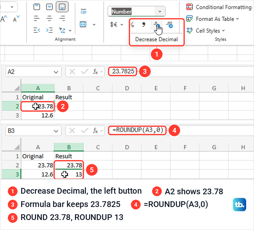
Formulas work the same way. Typing =ROUND( opened a card showing ROUND(number, num_digits) with a description, and =ROUND(A2,2) returned 23.78. =ROUNDUP(A3,0) turned 12.6 into 13, and A3 still read 12.6 afterwards. If you have not opened Excel in a browser before, our guide to using Excel for beginners shows where to find it.
Why a rounded number can look wrong
If a number looks rounded when you did not ask for it, or a rounding formula seems not to work, check these causes in order. The first three showed up on our sheet.
The column is too narrow
A General number rounds itself to fit a narrow column. When we dragged column A narrower, 25.76 showed as 26, and narrower still it showed a single #. The formula bar read 25.76 the whole time, and double-clicking the right edge of the column header brought the full number back.
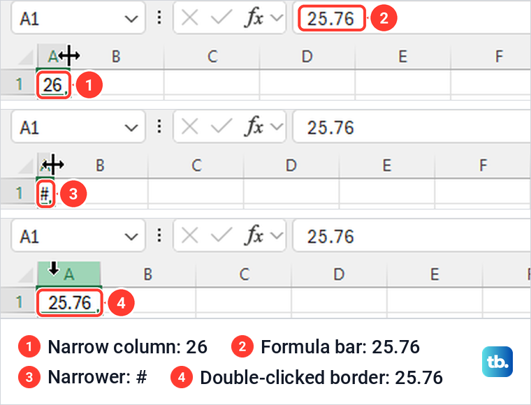
That is easy to mistake for real rounding. Microsoft gives the same fix, a double-click on the right border of the column header, for cells filled with # signs, and you can also resize and AutoFit columns by dragging their edge.
The formula shows as text
If a cell shows =ROUND(2.15,1) instead of 2.2, the cell was probably formatted as Text before you typed. On our sheet, switching the format back to General did nothing on its own. Pressing F2 and then Enter re-entered the formula and showed 2.2.
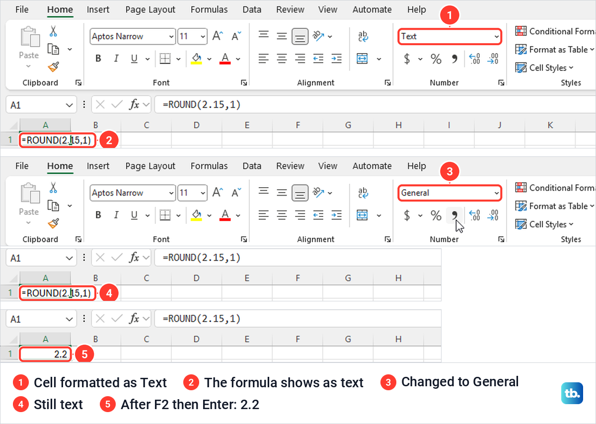
The other common cause is Show Formulas, which displays every formula on the sheet instead of its result. Turn it off under Formulas > Show Formulas or press Ctrl + `, the grave accent key. If neither helps, follow the fuller steps to fix Excel formulas showing as text.
The sheet is protected
On our protected sheet, which used the Protect Sheet defaults with Format cells unticked, the whole Number group on the Home tab was greyed out, and clicking Decrease Decimal did nothing. Typing in a cell brought up a message saying the cell is on a protected sheet. Review > Unprotect Sheet lifted it, after which Decrease Decimal showed 23.78 as usual.
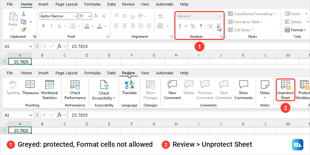
If the sheet has a password that is not yours, ask its owner, then unprotect the Excel worksheet with their permission. If you protect a sheet yourself, tick Format cells in the Protect Sheet box when others should still be able to change decimal places. Our guide to locking cells in Excel explains the other boxes.
Excel will not accept the commas
Formulas use a list separator between their parts, and Microsoft notes that the separator depends on your region and Excel settings. Where Excel expects semicolons, type =ROUND(A2;2) instead. If ROUND still returns an error after that, our guide to fix Excel functions that are not working goes through the other causes.
Set precision as displayed changes your data for good
Excel has a workbook setting that makes every number keep only the digits it shows. It sits under File > Options > Advanced, in the When calculating this workbook section, as Set precision as displayed. It was unticked in our new workbook.
We tried it on a separate practice workbook where A1 held 1.2345 shown as 1.23, and B1 doubled it to 2.469. Ticking the box raised one warning, Data will permanently lose accuracy, with only an OK button. After OK, the formula bar for A1 read 1.23 and B1 showed 2.46, so the hidden digits were gone from the data itself.
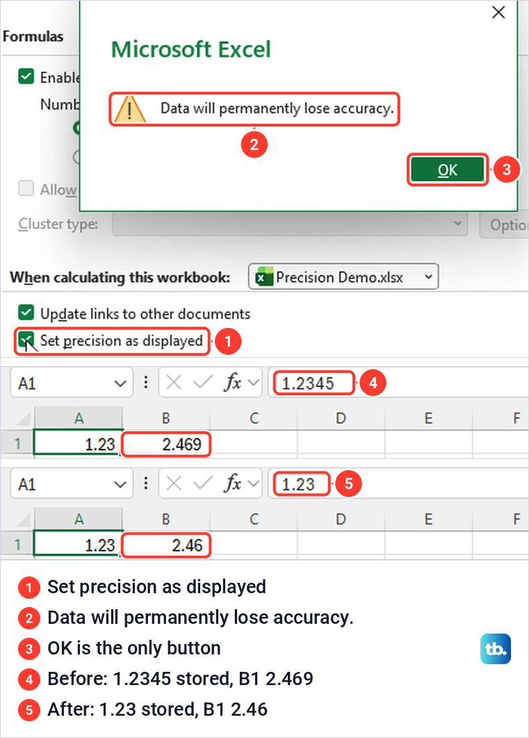
Microsoft warns that the original values cannot be restored if you later switch back to full precision, and that the option can make data less accurate over time. Round the cells that need it with ROUND instead, and if you do need this option, try it on a copy of the workbook first.
How we tested this guide
We tested this in Excel for Microsoft 365 on Windows 11, version 25H2, and in Excel for the web in Microsoft Edge, rounding a sheet of made-up numbers.
Frequently Asked Questions
How do I round to two decimal places in Excel?
To change only what you see, select the cells, press Ctrl + 1, choose Number and set Decimal places to 2. To get a rounded value for calculations, put =ROUND(A2,2) in another cell, which turned 23.7825 into 23.78 on our sheet while A2 kept its full value.
How do I round up a number in Excel?
Use ROUNDUP with the number of places to keep, such as 0 for a whole number. In our Excel for the web workbook, where A3 held 12.6, =ROUNDUP(A3,0) returned 13, and because ROUNDUP moves away from zero, a negative number becomes more negative.
How do I round down without changing the original cell?
Put =ROUNDDOWN(A2,0) or a similar formula in another cell. The original cell keeps its value, and only the formula cell holds the rounded result.
Why does Excel still calculate with decimals I cannot see?
Number formatting changes the display only, and calculations use the full stored value shown in the formula bar. Point your calculation at a ROUND result, or wrap the calculation itself in ROUND.
How do I round to the nearest 5 or 10 in Excel?
Use =MROUND(A2,5) or =MROUND(A2,10) for the nearest multiple, or =ROUND(A2,-1) for the nearest ten. When a positive number must always go up or down, use CEILING.MATH or FLOOR.MATH instead.
Why does my ROUND formula show 824 when I asked for two decimals?
The result cell has a format with fewer decimal places, often copied from the cell it refers to. Select it and set the format to General, and our 824 then showed as 823.78.
Can I round every number in a workbook permanently?
Set precision as displayed does that, but it changes stored values for good, and Microsoft says the originals cannot be restored by switching it off. It keeps only the digits each cell's format shows, so set the decimal places first and try it on a copy, though rounding the cells that need it with ROUND is the safer choice.