
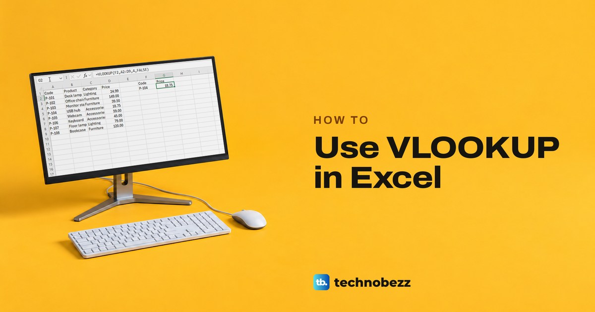
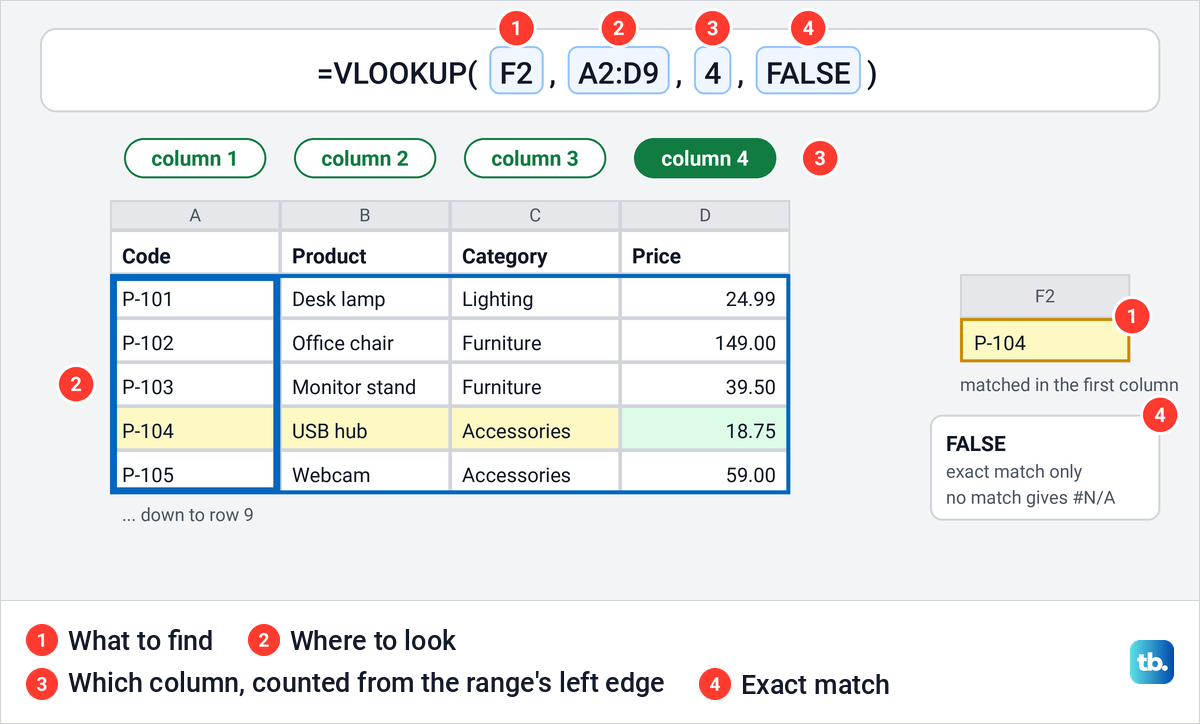
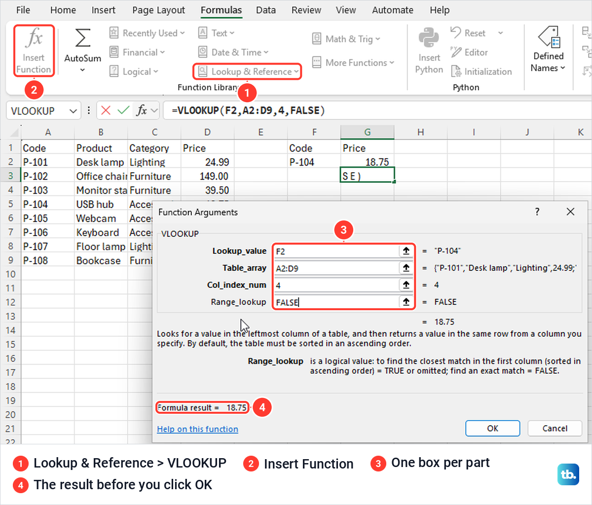
To use VLOOKUP in Excel, click the cell where the answer should go, type =VLOOKUP(F2,A2:D9,4,FALSE) and press Enter. The four parts are the value to find, the range whose first column holds it, the column number to bring back, and FALSE for an exact match. In our product list that formula returned 18.75, the price of product code P-104.
Two habits keep a VLOOKUP working. Lock the range with dollar signs before you fill the formula down, and remember that VLOOKUP can return a value from the column it searches or a column to its right, never from a column to its left. Leave out FALSE and Excel uses an approximate match by default, which can return a wrong answer with no warning.
We built the worked examples below in Excel for Microsoft 365 on Windows 11, version 25H2, using a made-up product list, and read each result back from the cell. The Excel for the web section repeats the key steps in Microsoft Edge.
The short version
- The formula: =VLOOKUP(what to find, where to look, column number, FALSE).
- Exact match: type FALSE as the last part unless you are looking up bands such as discounts or grades.
- Fill down safely: select the range in the formula and press F4 so it reads $A$2:$D$9.
- Not found: wrap the lookup in IFNA to show your own text instead of #N/A.
- Answer on the left: use XLOOKUP or INDEX and MATCH instead.
The VLOOKUP formulas in this guide
| What you want | Formula we used | What it returned |
|---|---|---|
| A price for a code on the same sheet | =VLOOKUP(F2,A2:D9,4,FALSE) | 18.75 for P-104 |
| Prices for an order list on another sheet | =VLOOKUP(B2,Products!$A$2:$D$9,4,FALSE), filled down | 18.75, 120, 24.99, #N/A, 149, 45 |
| The discount band for an order total | =VLOOKUP(D2,$A$2:$B$5,2,TRUE), filled down | 10% for an order of 260 |
| Your own text instead of #N/A | =IFNA(VLOOKUP(B5,Products!$A$2:$D$9,4,FALSE),"Not found") | Not found |
| A range that grows with new rows | =VLOOKUP(F2,ProductTable,4,FALSE) | 18.75, then 12 for a new row |
| A code that sits left of the product name | =XLOOKUP(F5,B2:B9,A2:A9) | P-105 for Webcam |
| A match on two columns at once | =VLOOKUP(F2,$A$2:$D$6,4,FALSE) with a helper key column | 13 for T-shirt M |
What the four parts of VLOOKUP mean
| Part | What it does | In our example |
|---|---|---|
| lookup_value | The value to find. It can be a cell, a number or text in double quotes | F2, which holds P-104 |
| table_array | The range to search. Its first column must hold the value you are looking for | A2:D9 |
| col_index_num | Which column of that range to return, counting its first column as 1 | 4, the Price column |
| range_lookup | FALSE for an exact match. TRUE, or leaving it out, gives an approximate match | FALSE |
The rule that trips most people up is in the second part. VLOOKUP only searches the first column of the range you give it, so the codes must sit in that column. Excel's own help line in the Function Arguments box puts it the same way, describing the value to find as the value to be found in the first column of the table.
The column number counts from the left edge of the range, not from column A. Our range A2:D9 makes Price column 4, but a range of B2:D9 makes Price column 3, because Product becomes column 1.
Write your first VLOOKUP formula
Our practice sheet, named Products, holds product codes in A2:A9, product names in column B, categories in column C and prices in column D. The code to look up goes in F2 and the answer in G2.
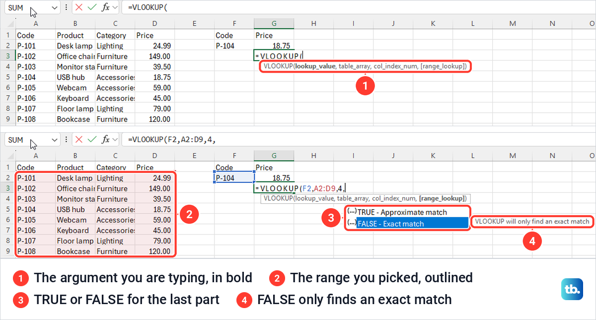
Click G2 and type =vl. Excel lists VLOOKUP with the tip Looks for a value in the leftmost column of a table, and then returns a value in the same row from a column you specify. Press Tab and Excel writes =VLOOKUP( for you, with a ScreenTip under the cell that lists the four parts and shows the one you are typing in bold.
Click F2, type a comma, then drag over A2:D9 and type another comma. Excel outlines each cell or range you pick in its own colour, an easy check that you grabbed the right rows. Type 4 and a comma, and Excel offers a short list with TRUE - Approximate match and FALSE - Exact match.
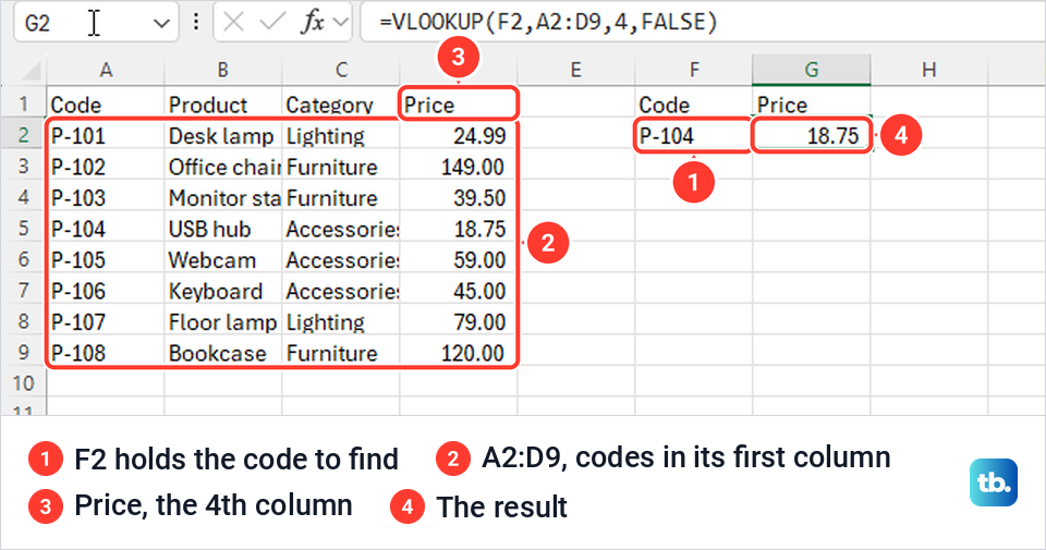
Choose FALSE, or type it, then type the closing bracket and press Enter. On our sheet G2 showed 18.75, and the formula bar showed =VLOOKUP(F2,A2:D9,4,FALSE) exactly as typed. Change the code in F2 and the answer follows it, so P-107 returned 79.
Our Price column was formatted with two decimals, yet G2 showed 79 rather than 79.00. VLOOKUP brings back the value, not the number format of the cell it came from, so format the answer cell yourself with the Number Format box on the Home tab.
Use the Function Arguments box instead of typing
If you would rather fill in boxes, click the answer cell, open Formulas > Lookup & Reference, scroll near the end of the list and choose VLOOKUP. On our PC, Insert Function on the same tab, the fx button beside the formula bar and Shift + F3 all opened the Insert Function dialog, where searching for vlookup and selecting Go lists it.
The Function Arguments box has one box for each part, a help line for the box you are in, and a live Formula result line. Ours showed 18.75 before we clicked OK, so a wrong column number shows up before the formula reaches the sheet. It also showed 18.75 while Range_lookup was still empty, which is a good reason to type FALSE anyway, because Excel was then doing an approximate match that happened to land on the right row.
Choose exact match or approximate match
The last part decides how VLOOKUP matches. FALSE finds only the exact value and returns #N/A when it is missing. TRUE, or leaving the part out, finds the largest value that is less than or equal to the one you look up, and Microsoft says the first column must then be sorted in ascending order.
Leaving it out is the trap. On our sheet =VLOOKUP(D3,$A$2:$B$5,2), with no fourth part, returned exactly what the TRUE version did. Microsoft's Excel blog lists that default as one of VLOOKUP's weak points, warning that if you forget, which is easy to do, you will probably get the wrong answer.
Type FALSE for codes, names and ID numbers. Keep TRUE for numbers that fall into bands, such as discount levels or grade boundaries, in a table sorted from smallest to largest.
Use approximate match for price bands
Our discount table lists where each band starts, so 50 gets 2%, 100 gets 5%, 250 gets 10% and 500 gets 15%. With order totals in D2:D6, we typed =VLOOKUP(D2,$A$2:$B$5,2,TRUE) in E2 and filled it down to row 6.
It returned #N/A for 20, 2% for 80, 5% for 100, 10% for 260 and 15% for 999. Each total lands in the last band it has reached, and 20 gives #N/A because it is below the first band. The FALSE version beside it returned #N/A for everything except 100, the only total that appears in the table.
If every total needs an answer, start the band table at 0, because =VLOOKUP(D2,$M$2:$N$6,2,TRUE) pointed at a copy with a 0 row returned 0 for the order of 20. Then format the results with Percent Style (Ctrl + Shift + 5), since VLOOKUP brought the discounts back as 0.02, 0.05, 0.1 and 0.15.
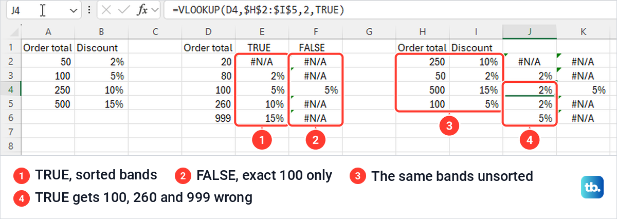
We copied the bands to H2:I5 in the order 250, 50, 500, 100 and pointed the same TRUE formula at the copy. It returned 2% for 100, 2% for 260 and 5% for 999, all wrong, with no error and no warning.
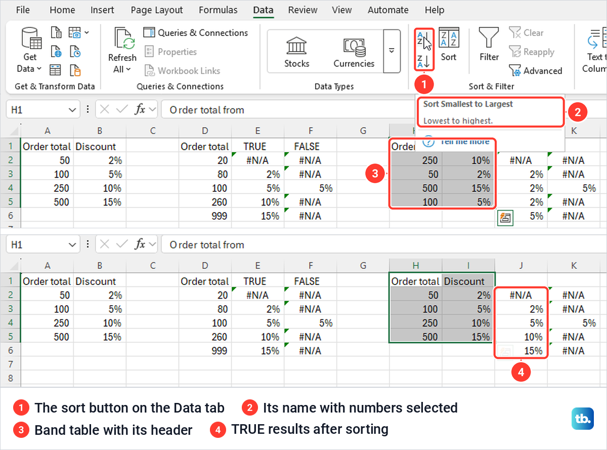
The fix is to sort. Select the band table with its header, open the Data tab and click the A to Z sort button, which Excel named Sort Smallest to Largest when numbers were selected. One click sorted our table under its header row, and the TRUE results matched the sorted table again.
Look up a value on another sheet
You do not need to type the other sheet's name. Excel writes it when you click that sheet's tab in the middle of a formula.
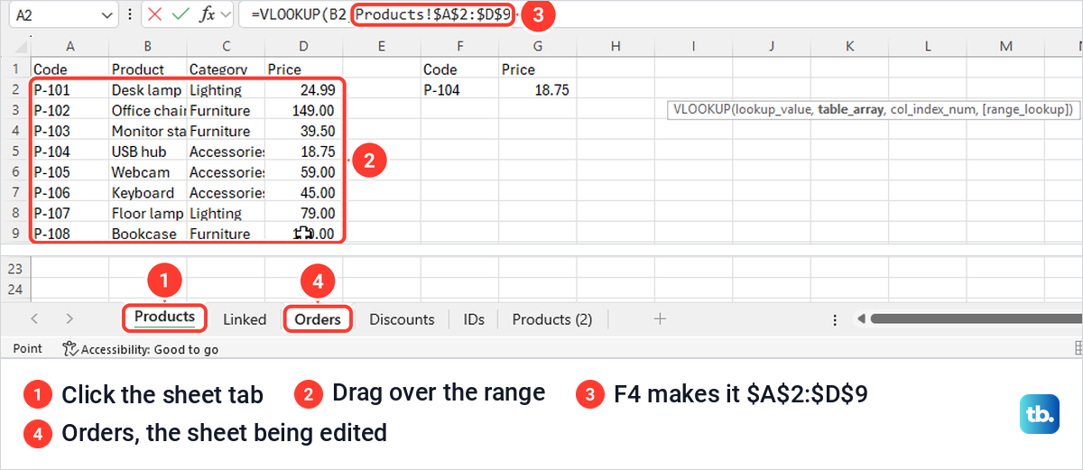
On our Orders sheet we typed =VLOOKUP(B2, in D2, clicked the Products tab and dragged over A2:D9. Excel wrote Products!A2:D9 by itself, and the Orders tab stayed highlighted as the sheet being edited. Pressing F4 right then turned the whole range into Products!$A$2:$D$9 in one press, ready for filling down.
Finish with ,4,FALSE) and press Enter. Our finished formula, =VLOOKUP(B2,Products!$A$2:$D$9,4,FALSE), returned 18.75 for code P-104.
Sheet names with spaces need single quotes. When we renamed Products to Product List, Excel rewrote the lookup as =VLOOKUP(B2,'Product List'!$A$2:$D$9,4,FALSE) and added the quotes itself, and renaming it back removed them. So rename sheets freely, but type the quotes yourself if you write a reference by hand.
Another sheet is also the natural home for a pick list. Put a drop-down list of product codes in the order sheet's Code column, and whoever fills it in picks a valid code while VLOOKUP brings in the price.
Lock the table range before you fill down
A VLOOKUP that works in one row often breaks when you copy it down. We filled our first Orders formula down to D7 without dollar signs and got 18.75, 120, #N/A, #N/A, #N/A and 45. P-101 and P-102 are both on the Products sheet, so two of those #N/A results were wrong.
D4 read =VLOOKUP(B4,Products!A4:D11,4,FALSE), because Excel moved the range down one row for every row it filled. From row 4 down, the range started below P-101 and P-102, so neither code could be found.
Click the first formula, select the whole A2:D9 text in the formula bar and press F4 once, so it reads $A$2:$D$9, then fill down again. Our locked version returned 18.75, 120, 24.99, #N/A, 149 and 45, and the only #N/A left was P-110, a code that is not in the list.
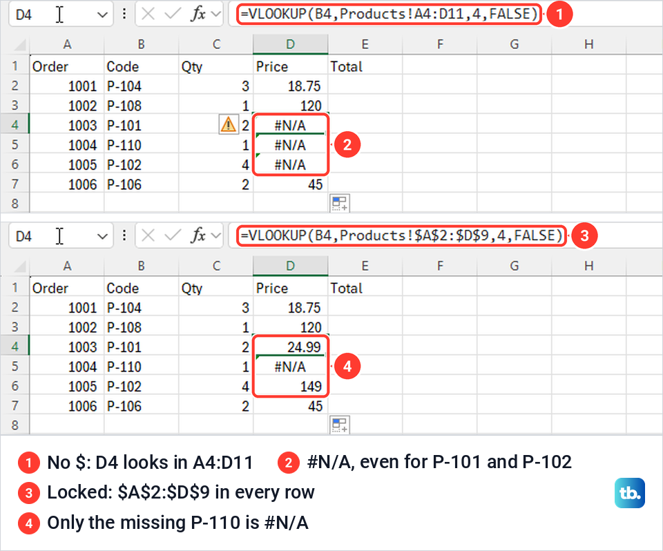
Select the whole range text first. When we only clicked inside the A2 half of the reference and pressed F4, Excel locked that half alone and stored Products!$A$2:D9, which leaves the end of the range free to move. Our guide to locking cells in Excel explains what each dollar sign does and how F4 cycles through them.
To fill down, double-click the small square at the bottom right of the cell. On our sheet it filled to D7 and stopped at the last row of data beside it, and selecting D2:D7 and pressing Ctrl + D did the same. F4 and Ctrl + D are two of the Excel keyboard shortcuts worth learning if you build lookups often.
Use an Excel table so new rows are included
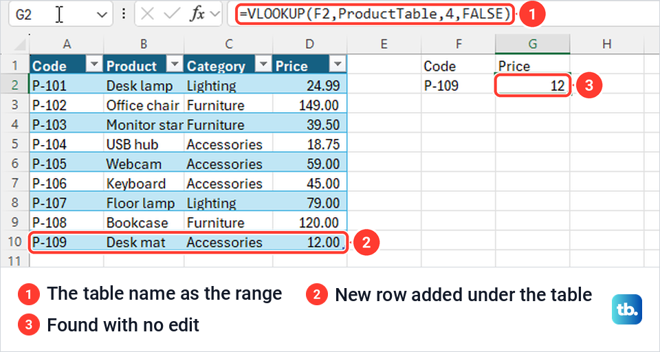
A fixed range such as $A$2:$D$9 does not grow when you add products under it, but an Excel table does. We selected the product list, chose Insert > Table and typed ProductTable in the box labelled What is the name of your table? before clicking OK.
While typing =VLOOKUP(F2,, we dragged over the table's data and Excel wrote the table name instead of cell addresses. The finished =VLOOKUP(F2,ProductTable,4,FALSE) returned 18.75. When we typed a new row under the table, P-109 Desk mat at 12, the table grew to include it and the same formula returned 12 for P-109 with no edit.
Look up a value in another workbook
The pointing method works across files too. Open both workbooks, start the formula in the one that needs the answer, and switch to the other one before you select the range. On our PC, View > Switch Windows worked in the middle of typing a formula and listed both open workbooks.
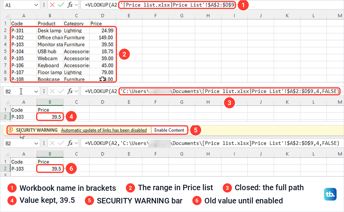
We typed =VLOOKUP(A2, in our practice workbook, switched to Price list.xlsx and dragged over A2:D9 on its Price List sheet. The formula bar showed '[Price list.xlsx]Price List'!$A$2:$D$9, with the file name in square brackets, single quotes because of the spaces, and dollar signs added automatically. After ,4,FALSE) and Enter, Excel returned us to the first workbook and the cell showed 39.5.
Our source file's only sheet had the same name as the file, and after Enter Excel stored the shorter =VLOOKUP(A2,'Price list.xlsx'!$A$2:$D$9,4,FALSE). When we closed the source, the formula showed the full folder path instead, from C:\Users\ through \Documents\[Price list.xlsx]Price List, and kept its value of 39.5.
When we changed the price in Price list.xlsx to 42 and reopened the practice workbook, a yellow bar read SECURITY WARNING Automatic update of links has been disabled, with an Enable Content button. The cell kept the old 39.5 until we clicked Enable Content, and then it showed 42.
To see every file a workbook draws from, open Data > Workbook Links in the Queries & Connections group. Our pane listed Price list.xlsx with a menu beside it, under Refresh all and Break all buttons that act on every link at once.
Show your own message instead of #N/A
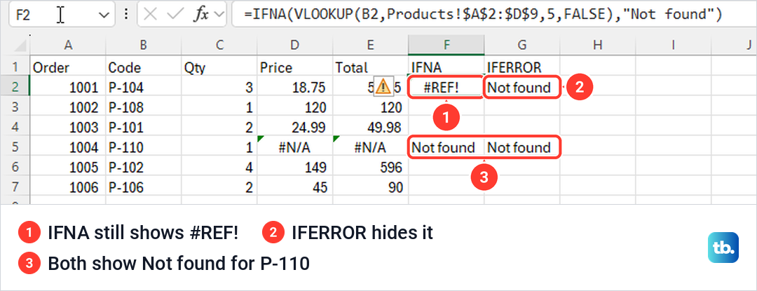
A missing code shows #N/A, which looks broken on an invoice or a report. Wrap the lookup in IFNA to show your own text instead. On our Orders sheet =IFNA(VLOOKUP(B5,Products!$A$2:$D$9,4,FALSE),"Not found") showed Not found for the missing P-110.
IFERROR does the same job but catches every error, and that is the problem. With the column number mistyped as 5 in a four-column range, our IFNA version still showed #REF!, while the IFERROR version showed Not found and hid the broken formula. Use IFNA for lookups, so a real mistake still shows up.
To leave the cell blank instead, use two double quotes as the last part. On our sheet =IFNA(VLOOKUP(B5,Products!$A$2:$D$9,4,FALSE),"") left an empty-looking cell for the missing code. Microsoft's function list dates IFNA to Excel 2013.
Things VLOOKUP does without warning you
With FALSE, it stops at the first match. We added a second P-104 row, USB hub (new) at 21.50, widened the range to A2:D10, and the formula still returned 18.75 from the first row. If a later copy should never win, remove duplicates from the lookup column first.
It ignores capitals, so p-104 typed in lower case still returned 18.75. Wildcards work with an exact match, and =VLOOKUP("Floor*",B2:D9,3,FALSE) returned 79 for Floor lamp. =VLOOKUP("*lamp",B2:D9,3,FALSE) returned 24.99 for Desk lamp, the first product ending in lamp.
Hidden columns still count. With column C hidden, the formula still needed column number 4 to return the price, so if a number seems off by one, unhide the hidden columns and count again. A decimal column number is cut down rather than rounded, and 3.9 returned Accessories from column 3 with no error.
Inserting a column inside the range is the worst case. When we inserted an empty column before Price, Excel widened the range to A2:E9 but kept the 4, so the lookup returned 0 from the new empty column. Once we typed Acme as a supplier in that column, it returned Acme instead of the price.
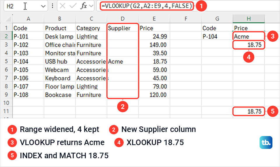
After the insert, the code cell had moved to G2 and Price to column E. =XLOOKUP(G2,A2:A9,E2:E9) and =INDEX(E2:E9,MATCH(G2,A2:A9,0)) both still returned 18.75. The same thinking applies if you move columns around inside the range, because the column number counts positions, not headings.
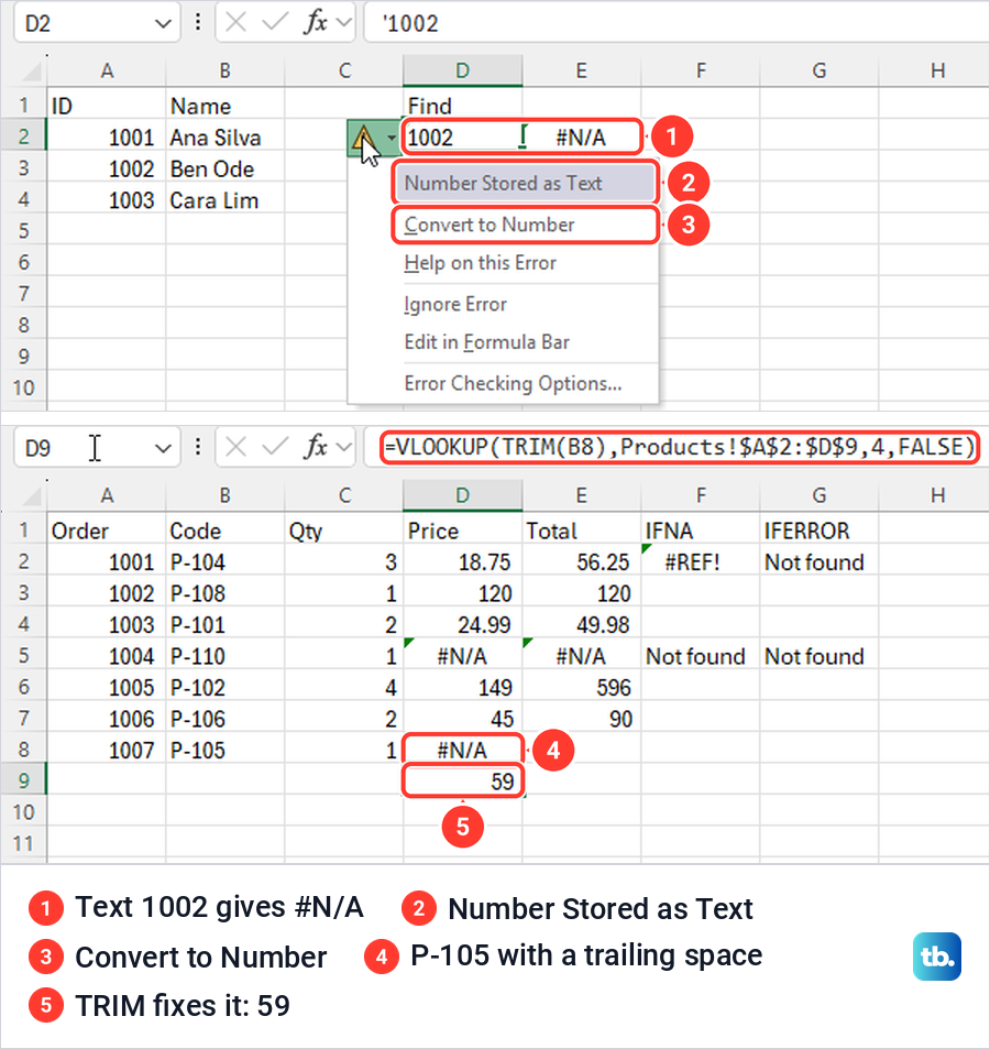
Numbers stored as text never match real numbers. In our ID list, 1002 typed as text gave #N/A against the numeric IDs, while the number 1002 returned Ben Ode. With the text cell selected, the error button beside it opened a menu headed Number Stored as Text, and Convert to Number fixed the lookup.
A trailing space does the same, and you cannot see it. A code pasted as P-105 with one space after it gave #N/A, while =VLOOKUP(TRIM(B8),Products!$A$2:$D$9,4,FALSE) returned 59. If the TRIM function is not working, the cell may hold a non-breaking space or a nonprinting character instead. Microsoft suggests the CLEAN function for nonprinting characters, and that guide covers both.
To match on two things at once, such as a product and a size, combine two columns into one key column at the left of the range. Our helper column used =B2&" "&C2 to build keys such as T-shirt M, and =VLOOKUP(F2,$A$2:$D$6,4,FALSE) with T-shirt M in F2 returned 13.
When the answer is to the left, use XLOOKUP or INDEX and MATCH
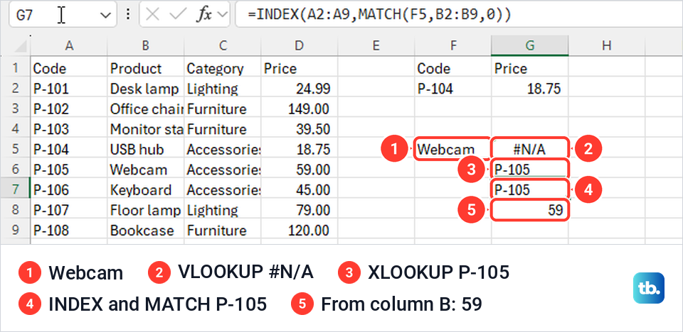
VLOOKUP can return a value from the column it searches or from a column to its right, but never from a column to its left. To find the code for Webcam, we typed Webcam in F5 and tried =VLOOKUP(F5,A2:D9,1,FALSE), which returned #N/A because Webcam is not in column A.
Two other formulas solved it. =XLOOKUP(F5,B2:B9,A2:A9) searches the Product column and returns from the Code column, and =INDEX(A2:A9,MATCH(F5,B2:B9,0)) does the same in two steps. Both returned P-105. When the answer is to the right of the column you search, VLOOKUP works again if the range starts at that column, and =VLOOKUP(F5,B2:D9,3,FALSE) returned 59, the price of Webcam.
| Question | VLOOKUP | XLOOKUP | INDEX and MATCH |
|---|---|---|---|
| Returns a value from the left | No | Yes | Yes |
| Match type when the last part is left out | Approximate | Exact | Approximate, so type 0 in MATCH |
| After a column is inserted in the range | Returned the wrong column on our sheet | Still returned 18.75 | Still returned 18.75 |
| Where it works, per Microsoft | All current versions, Mac and the web | Microsoft 365, Excel 2021 and later, Mac and the web | All current versions, Mac and the web |
Microsoft's Excel blog strongly recommends XLOOKUP for new work, while confirming that VLOOKUP will continue to be supported. XLOOKUP is not available in Excel 2016 or Excel 2019, so use VLOOKUP or INDEX and MATCH in workbooks opened in those versions.
Our guide on how to use XLOOKUP covers its not-found text and search options. If a Microsoft 365 copy of Excel does not offer XLOOKUP as you type, update Microsoft Office first, since Microsoft made it generally available in 2020.
VLOOKUP in Excel for the web and on a Mac
The same formula works in a browser. In Excel for the web in Microsoft Edge, =VLOOKUP(F2,A2:D9,4,FALSE) returned 18.75 on a copy of our product list, and =VLOOKUP(B2,Products!$A$2:$D$9,4,FALSE) filled down to the same six results as on the desktop. If you have not opened Excel in a browser before, our Excel for beginners guide shows where to find it.
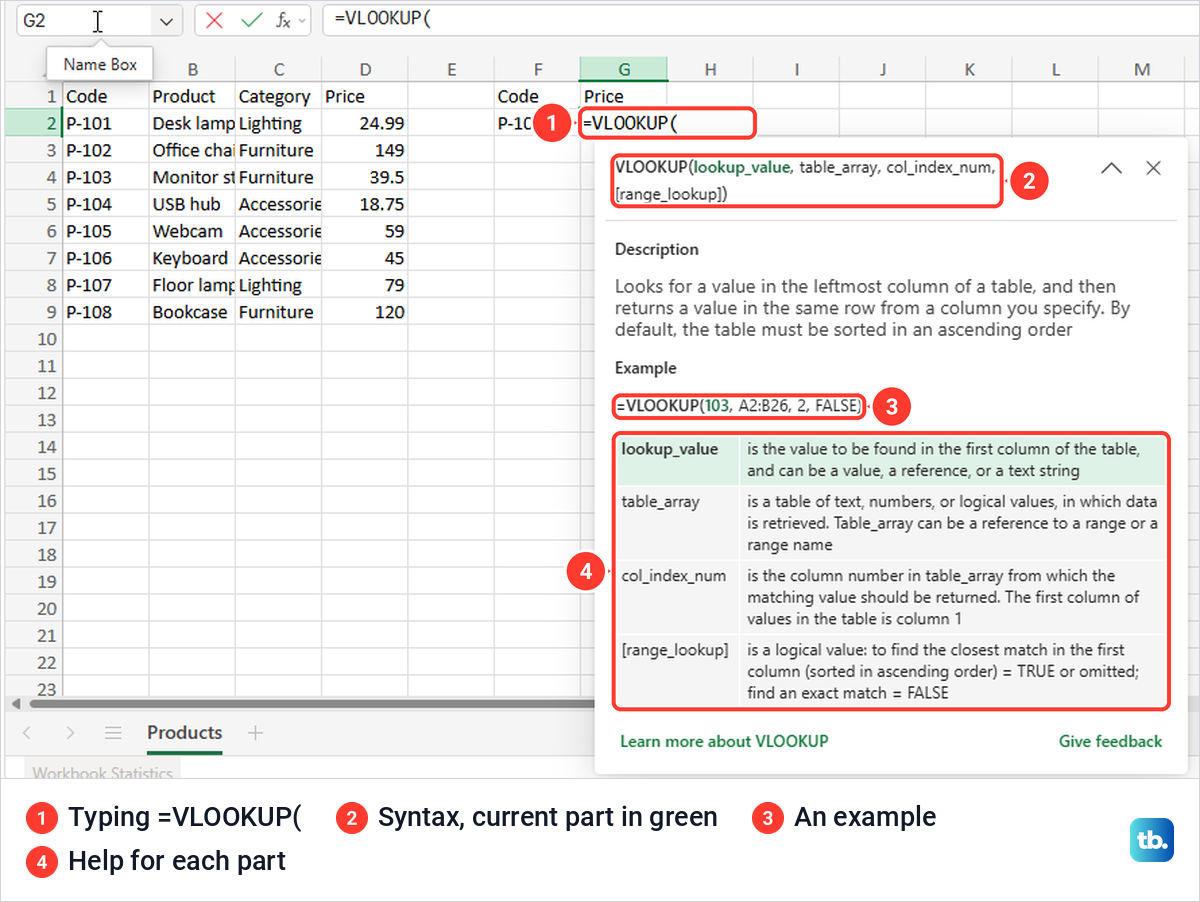
Typing =vl showed VLOOKUP with the shorter description Returns the first search result in a vertical list, and pressing Tab opened a larger card with a description, an example and help for each part. Pointing at another sheet first wrote 'Products'!A2:D9 with quotes, which Excel for the web dropped once we pressed Enter.
F4 worked in Edge too, and with the cursor inside A2 it locked only that half, as on the desktop. The first press showed a tip headed Excel shortcuts enabled, which says you can hand the browser shortcuts back under Help > Keyboard Shortcuts.
Another workbook works in Excel for the web as well, even though it is often described as a desktop-only job. With one workbook's formula half typed, we switched to a second browser tab holding the price list and dragged over A2:D9. Excel showed a bar asking us to select a range to apply to the formula in Orders web.xlsx, and wrote the other file's full OneDrive address into the formula.
Back in the first tab, we finished the formula with ,4,FALSE) and pressed Enter. The cell showed #N/A under a bar asking Trust workbook links?, and selecting Trust Workbook Links made it return 39.5. Microsoft's help page calls this step Enable Content, and it says both workbooks must be saved in an online location you can reach with your Microsoft 365 account.
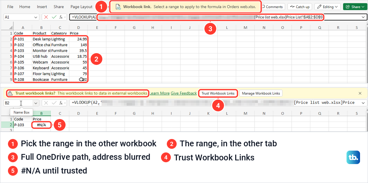
When we reopened that workbook, the same bar appeared, but the cell already showed the saved 39.5. Trusting a link also opens a Workbook Links pane. Its Settings tab has an Always trust workbook links switch, which was off on our account, and its tip says turning it on remembers your choice for that workbook.
Excel for Mac uses the same formula. To switch a selected reference to absolute there, Microsoft gives Command + T, and its Mac shortcut list names F4 as well.
When VLOOKUP shows an error
#N/A means the value was not found in the first column of the range, for one of the reasons above. A wrong value with no error can mean the last part is TRUE or missing on an unsorted list, a column inserted inside the range or a duplicate code, all covered above.
#REF! appeared on our sheet when the column number was larger than the number of columns in the range, 5 for our A to D range. Count the columns again from the left edge of the range.
A column number of 0 gave #VALUE! on our sheet, and the error button beside the cell was headed The column index is too small. Microsoft adds that a value to find longer than 255 characters also causes it.
#NAME? appeared when we typed text without quotes, as in =VLOOKUP(Webcam,Products!$B$2:$D$9,3,FALSE), and the error button read Invalid Name Error. Put text inside straight double quotes, such as "Webcam".
If a cell shows the formula itself instead of a result, one cause is a cell formatted as Text before you typed. That is what happened on our sheet, where the formula showed with a green triangle, and our guide to formulas showing as text covers this and the other causes. For anything else, our guide to fix a VLOOKUP that is not working goes through recalculation, broken workbook links and the rarer causes one by one.
How we tested this guide
We tested this in Excel for Microsoft 365 on Windows 11, version 25H2, typing the worked examples into a practice workbook of made-up data.
Frequently Asked Questions
What does FALSE mean in a VLOOKUP formula?
It asks for an exact match, and VLOOKUP returns #N/A if the value is not in the first column. TRUE, or leaving the last part out, asks for an approximate match, which needs the first column sorted from smallest to largest.
Why does VLOOKUP return #N/A when I can see the value?
Usually the value is text on one side and a number on the other, has a stray space, or is not in the first column of the range. On our sheet, Convert to Number fixed the first case and TRIM fixed the second.
Can VLOOKUP look to the left?
No. It returns values from the column it searches or a column to its right, never one to its left, so use XLOOKUP or INDEX and MATCH, which both found the code to the left of the product name on our sheet.
How do I use VLOOKUP with another sheet?
Start the formula, click the other sheet's tab and drag over the range. Excel adds the sheet name and an exclamation mark, with quotes if the name has a space, and pressing F4 straight away locks the range.
What does VLOOKUP do if the value appears twice?
With FALSE, it returns the first matching row from the top. Our duplicate code returned the first row's price, not the later one.
Is VLOOKUP case-sensitive?
No. A lower-case p-104 found P-104 on our sheet and returned the same price.
Does VLOOKUP work in Excel for the web?
Yes. The basic lookup, the other-sheet lookup and the IFNA version returned the same results in Excel for the web, and a lookup into a second online workbook worked once we selected Trust Workbook Links.