


To multiply in Excel, type an equal sign, the first number or cell, an asterisk (*) and the second number or cell, then press Enter. On our sheet =5*10 returned 50, and =B2*C2 multiplied a quantity of 2 by a price of 5 to return 10. The asterisk is the multiplication sign Excel understands, and typing the letter x instead gives an error rather than an answer.
The right method depends on the job. Fill one formula down to multiply two columns row by row, lock a single cell with dollar signs to multiply a column by a number, use PRODUCT for several factors, and use Paste Special in desktop Excel when the existing numbers themselves should change. Excel for the web, Mac and phones follow after the desktop steps.
The short version
- Type
=5*10or=B2*C2and press Enter. The asterisk multiplies, the letter x does not. - Fill
=B2*C2down with the fill handle or Ctrl + D to multiply two columns. - Press F4 right after typing E2 to make it $E$2, so every row uses the same multiplier.
- Use
=PRODUCT(B2:B4)to multiply a whole range at once. - Paste Special > Multiply, opened with Ctrl + Alt + V, changes typed numbers themselves and leaves no formula.
Ways to multiply in Excel at a glance
Every method below except Paste Special leaves a formula in the cell, so the answer follows its numbers when they change. Paste Special overwrites the typed numbers you select with the products and keeps no formula. The results come from our practice sheet of made-up quantities and prices.
| Method | Use it for | Result on our sheet |
|---|---|---|
Type =5*10, then Enter | Two numbers you already know | 50 |
Type =B2*C2, then Enter | Two cells, such as a quantity and a price | 10, and it changes when either cell changes |
| Drag the fill handle or press Ctrl + D | Two whole columns, row by row | 10, 28 and 12 |
Press F4 to write =B2*$E$2 | A column times one fixed number | 6, 12 and 18 |
Type =PRODUCT(B2:B4) | Several cells or a whole range | 48 |
| Paste Special > Multiply, opened with Ctrl + Alt + V | Changing typed numbers in place in the desktop apps | 10, 20 and 30 became 20, 40 and 60 |
Type =B2*C2*10% | A percentage of a result | 1, ten percent of 10 |
Multiply two numbers in one cell
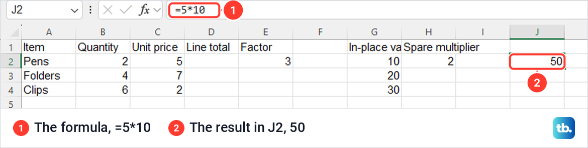
Click an empty cell, type =5*10 and press Enter. The cell shows 50, and when you click it again the formula bar above the column letters shows =5*10. That bar is the quickest way to check what a cell really holds, because the cell itself only shows the answer.
On a full-size keyboard the asterisk is the * key on the number pad, and on a US layout it is also Shift + 8. For more than two numbers, keep adding an asterisk and the next number before you press Enter.
Multiply two cells
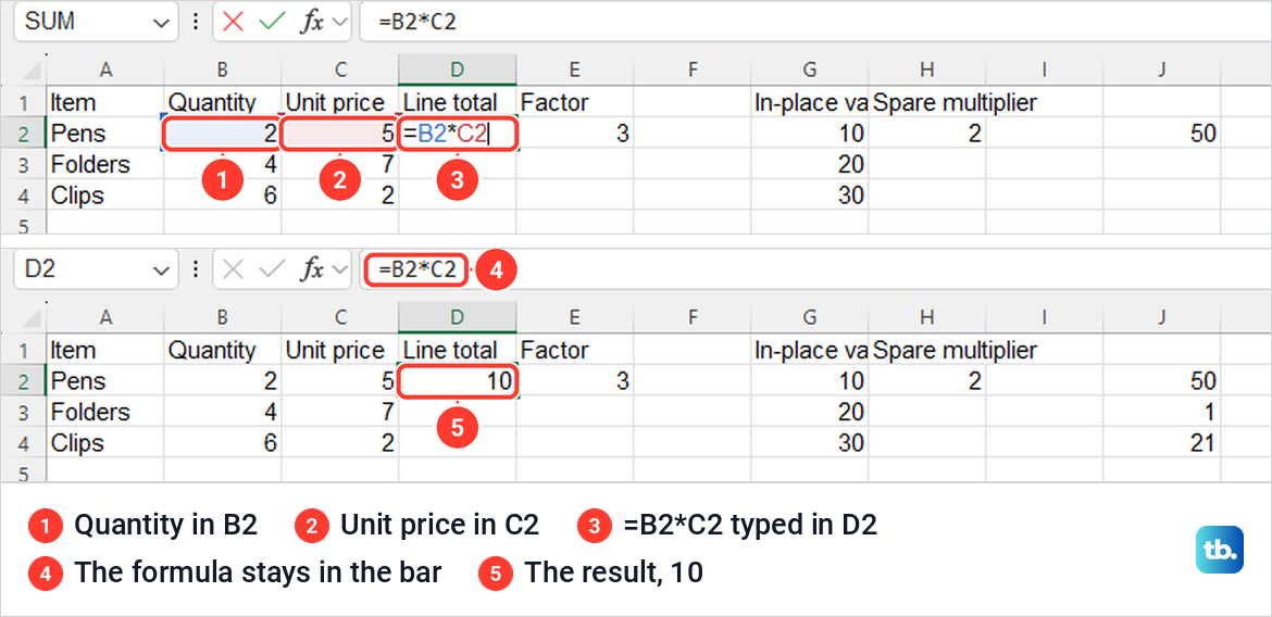
Our sheet lists items with a quantity in column B and a unit price in column C, and the line total goes in column D. Click D2, type an equal sign, click B2, type an asterisk, click C2 and press Enter. Typing =B2*C2 does the same, and while you type, Excel outlines each cell the formula uses in its own colour.
On our sheet D2 showed 10, the quantity of 2 times the price of 5. Because the cell holds a formula rather than a typed number, the result follows B2 and C2 whenever either one changes, as long as calculation is set to Automatic. The fixes near the end show what happens when it is not.
Multiply two columns row by row
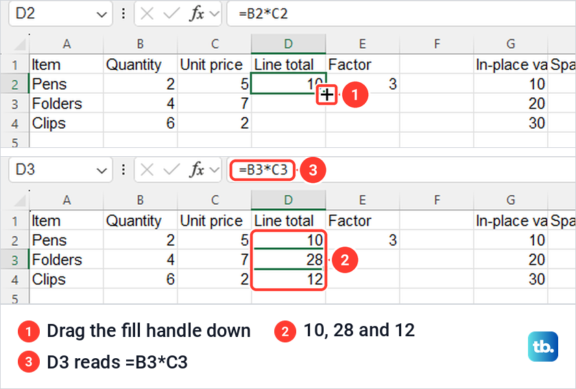
To get a line total for every row, write the formula once and copy it down. Click D2, which holds =B2*C2, and point at the small square at its bottom right corner until the pointer turns into a thin black cross. Drag it down to the last row of data and let go.
Our three rows filled with 10, 28 and 12, and clicking D3 showed =B3*C3 in the formula bar. Excel moved both cell references down one row for each row it filled, which is what you want when every row has its own quantity and price. Microsoft calls these relative references, and they change whenever a formula is copied.
If you would rather not drag, select the formula cell and the empty cells under it, then press Ctrl + D. With D2:D4 selected that filled the same 10, 28 and 12 on our sheet, and D4 read =B4*C4. Microsoft also shows double-clicking the fill handle, which copies the formula down beside a filled column in one go.
When the list grows, insert another Excel row inside the data and fill the formula into it. If dragging copies the same number into every cell or stops early, fix the Excel fill handle before you redo the column.
Multiply a column by the same number
Sometimes every row needs the same multiplier, such as a markup or an exchange rate. Put the multiplier in a cell of its own, which on our sheet was 3 in E2, under a Factor heading. The formula then needs one reference that moves down the rows and one that stays put.
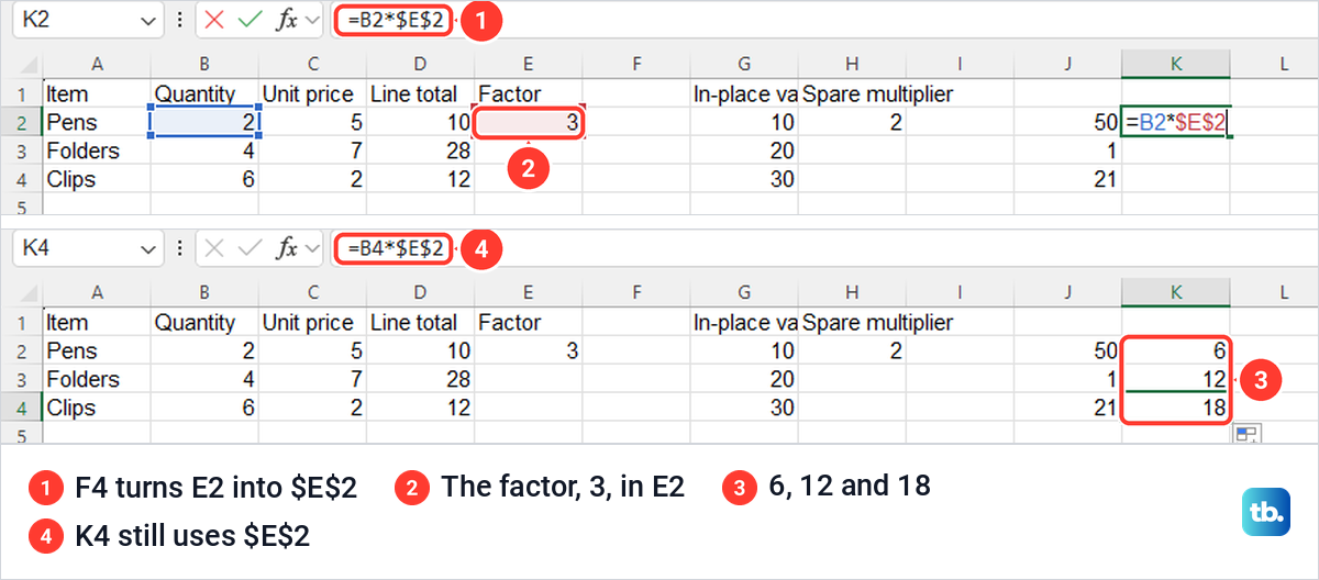
Click K2 and type =B2*E2, then press F4 once while the cursor sits right after E2. Excel changed it to =B2*$E$2 on our sheet, and the two dollar signs lock both the column and the row. Press Enter and fill the formula down as before.
Our column filled with 6, 12 and 18, and K4 read =B4*$E$2. The quantity reference moved down each row while the multiplier stayed on E2. To lock only the row or only the column, our guide to locking cells and references in Excel shows what each press of F4 does, and what to press on a Mac or when F4 changes a laptop's volume or brightness.
Why a copied formula shows 0
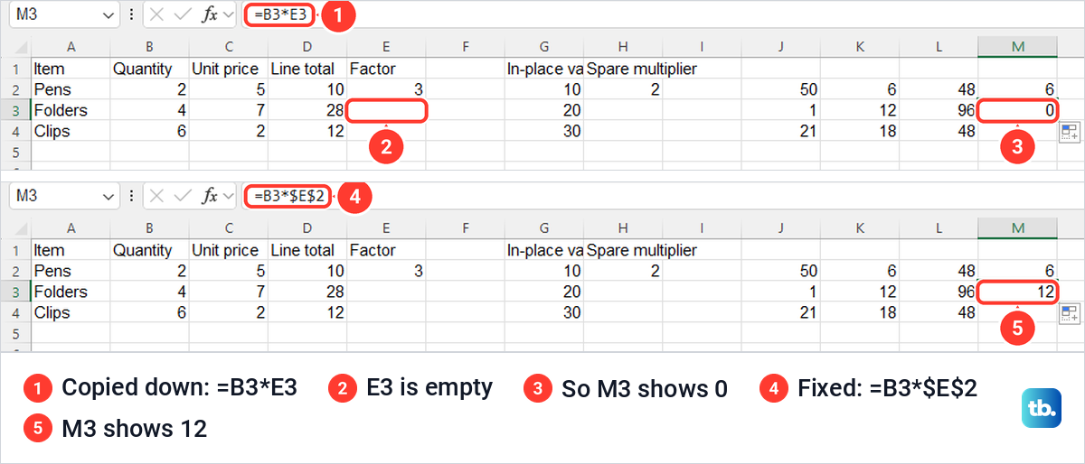
Leave out the dollar signs and the multiplier moves too. We filled =B2*E2 down from M2, and M3 became =B3*E3. E3 was empty, and M3 showed 0 with no error and no warning.
Clicking a suspicious zero and reading the formula bar is the quickest check. After we changed the formula to =B2*$E$2 and filled it again, M3 read =B3*$E$2 and showed 12.
Multiply several cells with PRODUCT
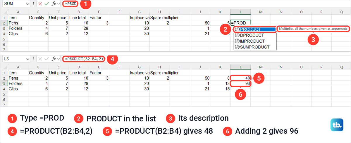
For more than two factors, the PRODUCT function saves typing an asterisk between each one. Type =PROD and Excel lists PRODUCT, DPRODUCT, IMPRODUCT and SUMPRODUCT, with the tip "Multiplies all the numbers given as arguments" beside PRODUCT. Pick PRODUCT, then add the range and a closing bracket.
On our sheet =PRODUCT(B2:B4) multiplied 2, 4 and 6 to return 48, and =PRODUCT(B2:B4,2) returned 96, because the extra argument 2 doubled the result. Microsoft says PRODUCT takes up to 255 arguments, and each one can be a number, a cell or a range.
One difference matters before you swap an asterisk for PRODUCT. Microsoft says PRODUCT ignores empty cells and text inside a range, while on our sheet an empty cell made an asterisk formula return 0 and a text cell made one return #VALUE! instead. PRODUCT is more forgiving of gaps, but it can also leave out a value someone typed as text without telling you.
Use the Function Arguments box
If you prefer boxes to typing, click the answer cell and press Shift + F3, or click Insert Function at the left end of the Formulas tab. In the Insert Function dialog, search for product, select PRODUCT and click OK. Its description reads "Multiplies all the numbers given as arguments".
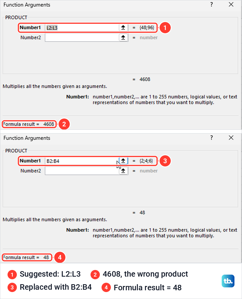
Check the range before you click OK. In L4, under two PRODUCT results, the Function Arguments box filled Number1 with L2:L3 by itself and showed a Formula result of 4608, the product of those two answers. We replaced it with B2:B4, the preview changed to 48, and OK put 48 in the cell.
Multiply existing numbers with Paste Special
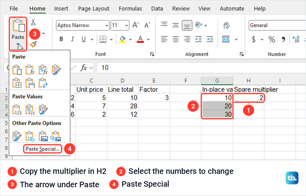
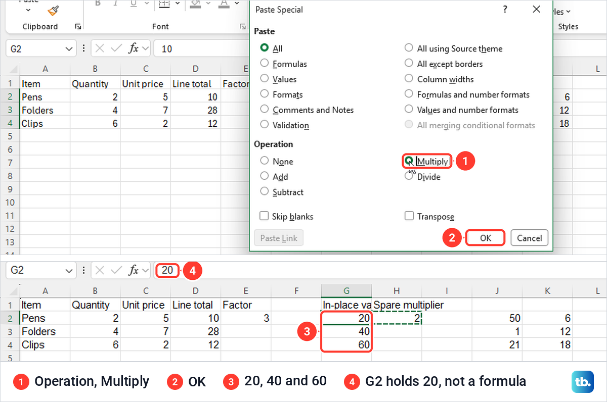
Paste Special changes numbers where they sit, without a helper column or a formula. It suits a one-off job such as doubling a column of prices you will not need to recalculate. Our example doubles the values 10, 20 and 30 in G2:G4 using a 2 in H2.
Select the multiplier cell, H2, and press Ctrl + C to copy it. Select the numbers you want to change, then on the Home tab click the arrow under Paste and choose Paste Special at the bottom of the menu.
In the Paste Special box, choose Multiply under Operation and click OK. The box opens with Paste set to All, which Microsoft says pastes all cell contents and formatting of the copied data, so choose Values under Paste as well if the numbers should keep their own formatting.
On our sheet the three cells became 20, 40 and 60. Clicking G2 showed 20 in the formula bar, a plain number with no formula, so the values no longer depend on H2.
Ctrl + Alt + V opened the same Paste Special box directly, and so did right-clicking the selection and choosing Paste Special, and both routes gave 20, 40 and 60. To go back, press Ctrl + Z straight away, which restored 10, 20 and 30 for us.
If the copied value never reaches the dialog, fix Excel paste problems first. F4, Ctrl + D and Ctrl + Alt + V are three of the Excel keyboard shortcuts worth learning if you multiply columns often.
Multiply by a percentage
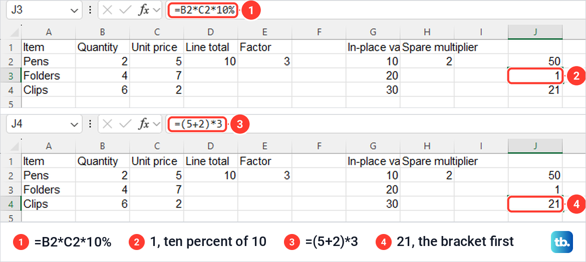
Excel reads the percent sign as part of the number, so 10% counts as 0.1. On our sheet =B2*C2*10% returned 1, which is ten percent of the 10 line total. Multiplying by a percentage gives you that share of the number, not the number raised or lowered by it.
To raise a value by a percentage, multiply it by one plus the rate, and to lower it, multiply by one minus the rate. Microsoft's own example uses =113*(1+0.25) for a 25 percent increase, which gives 141.25, and =113*(1-0.25) for a 25 percent decrease, which gives 84.75. The same pattern works with a cell, such as =B2*(1+10%).
The brackets matter, because Excel multiplies before it adds. Microsoft's example =5+2*3 returns 11, while our =(5+2)*3 returned 21 because the bracket was worked out first. To compare an old figure with a new one, calculate percentage change in Excel, and to take a fixed amount off every value, subtract values in Excel instead.
Multiply in Excel for the web
The same formulas work in a browser. In Excel for the web in Microsoft Edge, =B2*C2 returned 10 and =PRODUCT(B2:B4) returned 48 on a copy of our numbers, and typing =PROD suggested PRODUCT with the same description as the desktop app. If Excel itself is new to you, our Excel for beginners guide covers the basics.
A workbook only accepts changes while it is in Editing. The button at the top right of the web app switches between Editing (Make any changes) and Viewing (View the file, but make no changes), and the same menu offers Open in Desktop. Our new workbook opened in Editing.
Excel for the web adds a Multiply entry to the AutoSum list on the Formulas tab, beside Add, Minus and Divide. Select the cell for the answer, open the Formulas tab, click the arrow under AutoSum and choose Multiply.
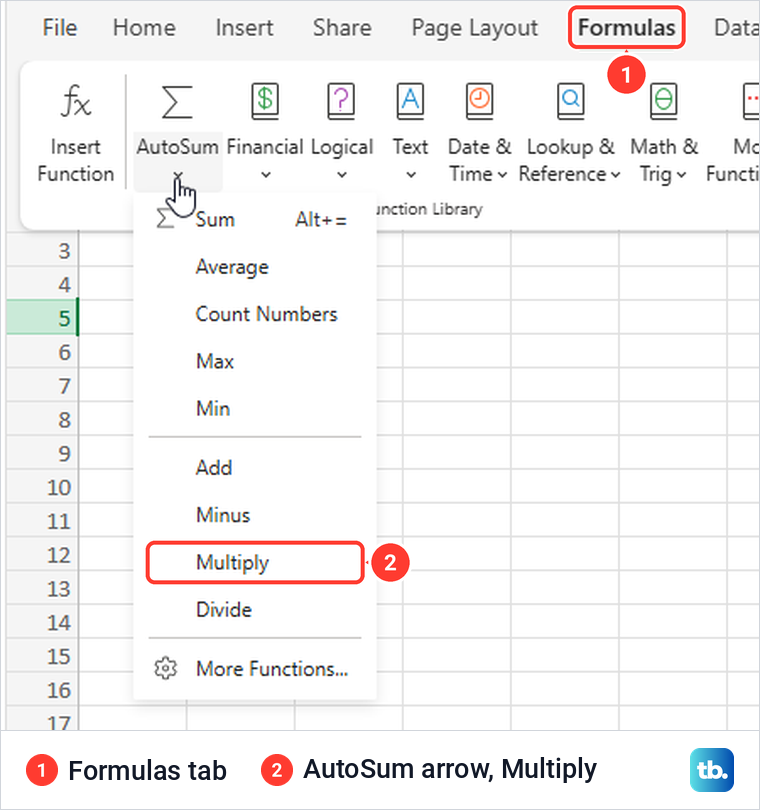
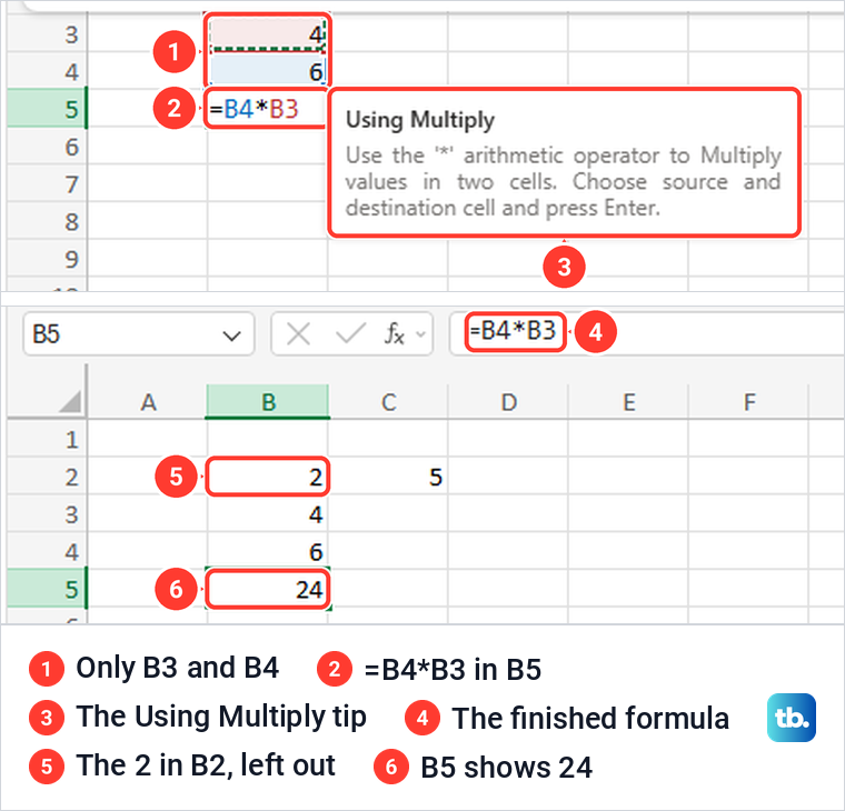
With B5 selected under 2, 4 and 6, it wrote =B4*B3, the two cells directly above, and showed a tip headed "Using Multiply". After we confirmed it, B5 showed 24, so the helper multiplied two cells and left the 2 in B2 out.
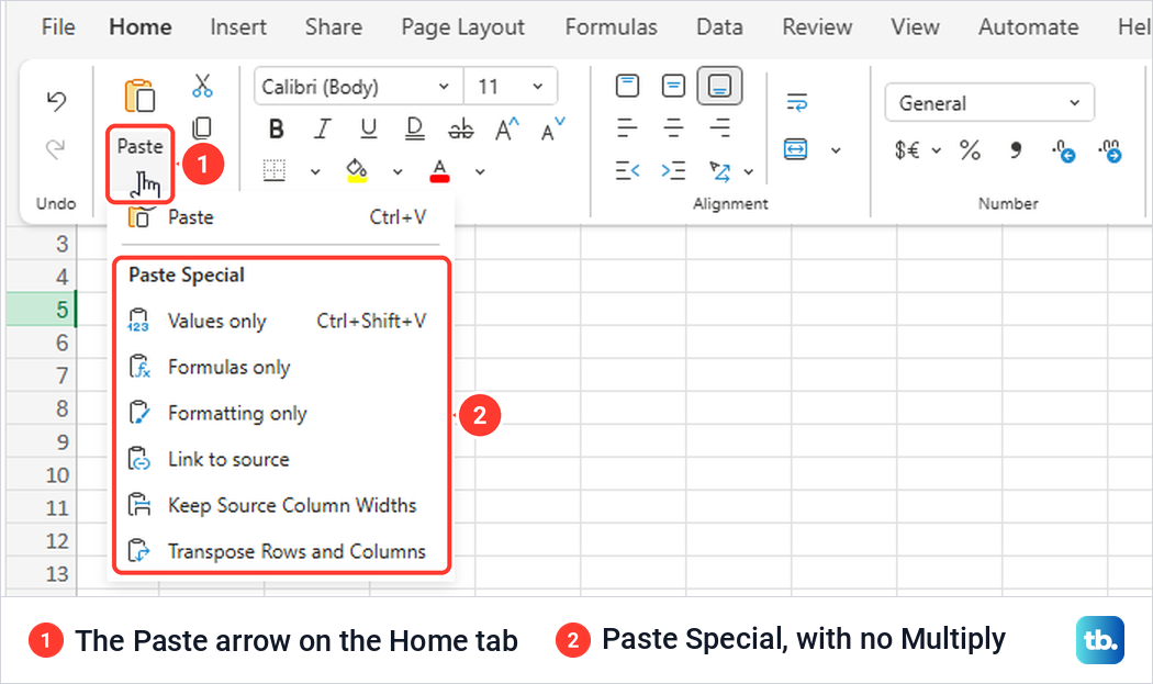
The web Paste menu had no Multiply option. After we copied a cell, it listed Values only, Formulas only, Formatting only, Link to source, Keep Source Column Widths and Transpose Rows and Columns, with no Multiply or other arithmetic option. In the browser, use a formula in a spare column, or choose Open in Desktop and use Paste Special there.
Multiply on a Mac, iPhone or Android phone
Excel for Mac uses the same asterisk formulas and the same PRODUCT function. Its Paste Special works the same way too: on the Home tab, select the arrow next to Paste, then Paste Special, and choose Multiply, which Microsoft describes as multiplying the values in the paste area by the values in the copy area.
On an Android phone, Microsoft says to tap the formula bar, type the formula and tap the check mark, or tap the fx button to start a function such as PRODUCT. Microsoft's iPhone guide says to double-tap the cell or tap in the formula bar, then type the formula with an asterisk between the cells.
When the product is wrong or missing
A broken multiplication shows up as an error, a zero, the formula itself or an old number that will not change. Click the cell and read the formula bar first, because it shows exactly what Excel is multiplying.
The letter x gives #NAME?
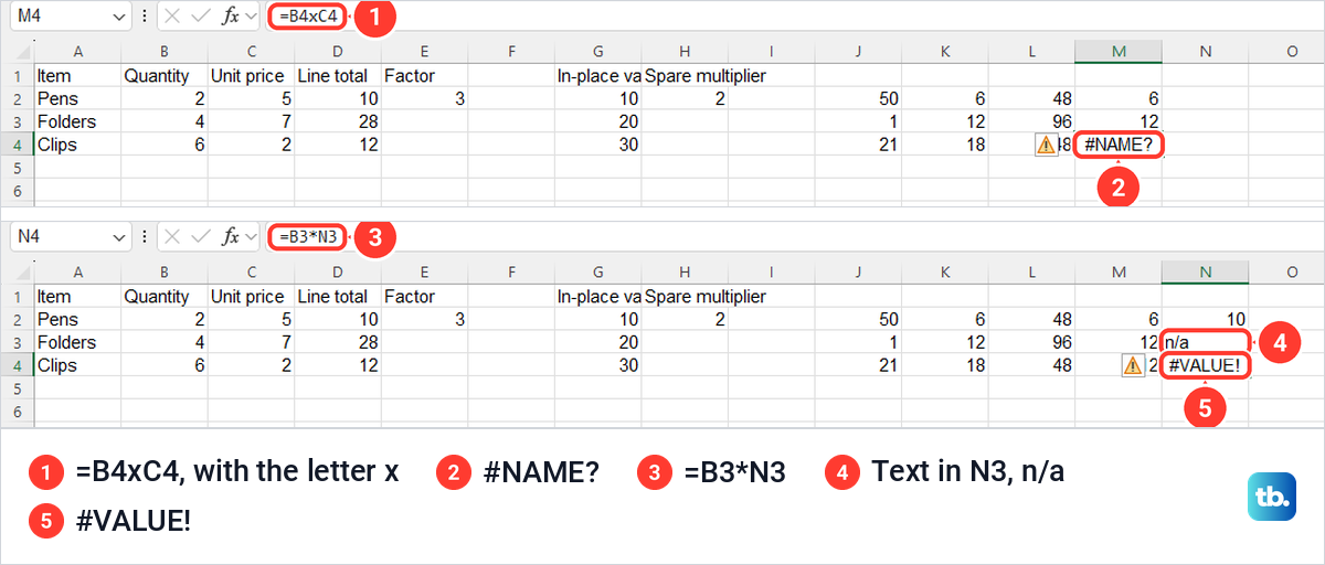
Excel does not treat the letter x as a multiplication sign. We typed =B4xC4, Excel accepted it without any prompt, and the cell showed #NAME? straight away. Replacing the x with an asterisk, =B4*C4, returned 12.
Text in a factor cell gives #VALUE!
A cell that holds text, such as a note reading n/a, breaks an asterisk formula. With n/a in N3, =B3*N3 showed #VALUE! on our sheet, and typing 7 into N3 turned it into 28. A stray space in a cell that looks empty is text too, so clear the cell or type the number again.
The formula shows instead of the answer
If one cell displays =B2*C2 exactly as typed, one cause is a cell formatted as Text before the formula went in. That is what a Text-formatted cell did on our sheet. Set the cell's format to General in the Number group on the Home tab, then press F2 and Enter to enter the formula again. Ours then returned 10.
If every formula on the sheet shows at once and the columns look wider, Show Formulas is on. It sits in the Formula Auditing group of the Formulas tab, where it can appear as an icon without a label, and its tooltip reads "Show Formulas (Ctrl+`)". Pressing Ctrl + ` switched our sheet back to results. For the other causes, see how to fix formulas showing as text.
The answer does not update
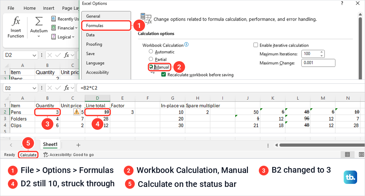
If you change a number and the product stays the same, check whether calculation is set to Manual. Open File > Options > Formulas and look at Workbook Calculation, which offered Automatic, Partial and Manual on our PC. The Calculation Options button at the right end of the Formulas tab is a quicker way to the same setting. With Manual selected we changed B2 from 2 to 3, and D2 stayed at 10.
Excel did flag it. The old 10 was drawn struck through with a small green triangle in the corner, every other dependent result looked the same, and the status bar showed Calculate. Selecting Automatic again recalculated the sheet at once, and D2 showed 15. If calculation is already Automatic, our guide to fix formulas that do not update covers the other causes.
Excel will not let you type the formula
A protected sheet blocks the edit with a message that begins "The cell or chart you're trying to change is on a protected sheet". Ours had no password, so Review > Unprotect Sheet removed the protection and =B2*C2 then returned 10. If the sheet has a password you know, unprotect the Excel worksheet with it, and turn protection back on afterwards if the file is shared.
How we tested this guide
We tested this in Excel for Microsoft 365 on Windows 11, version 25H2, and in Excel for the web in Microsoft Edge, multiplying a small made-up price list.
Frequently Asked Questions
What is the multiplication symbol in Excel?
It is the asterisk (*). Type =5*10 and press Enter to get 50, or use cell addresses such as =B2*C2 to multiply cells.
How do I multiply two columns in Excel?
Type =B2*C2 in the first row of an empty column, then drag the fill handle down or select the cells and press Ctrl + D. Each row multiplies its own pair of cells, so row 3 uses B3 and C3.
How do I multiply a whole column by one number?
Put the number in its own cell and lock that cell in the formula, such as =B2*$E$2, before you fill it down. Pressing F4 right after typing E2 adds the dollar signs.
Can I multiply numbers without adding a new column?
Yes, in the desktop apps. Copy the multiplier, select the typed numbers, open Paste Special, choose Multiply and click OK, and Excel replaces them with the products.
Why does my multiplication formula return 0?
An empty factor cell gave us 0 with no warning. After copying a formula, check the formula bar, because an unlocked multiplier reference may have moved to a blank cell.
Why do I get #VALUE! when I multiply?
A referenced cell that holds text instead of a number is one possible cause, so check the cells the formula uses. On our sheet a cell reading n/a caused it, and typing a number in its place fixed it.
Can I use Paste Special Multiply in Excel for the web?
Not from the Paste menu. When we tried it, the Paste menu in Excel for the web offered values, formulas, formatting, links and transpose options but no Multiply, so use a formula such as =B2*C2 or open the file in the desktop app.