
To strikethrough in Excel on Windows, select the cell or range and press Ctrl + 5. Press the same keys again and the line goes away, while the text in the cell stays exactly as it was. The other way to strike through text is the Format Cells box, where Strikethrough sits under Effects.
On our PC, the desktop Home tab had Bold, Italic and Underline buttons but no Strikethrough button, so the shortcut and the Format Cells box are the everyday routes there. Excel for the web is different and does show a Strikethrough button.
The short version
- Windows shortcut: select the cells and press Ctrl + 5. Press it again to remove the line.
- One word only, on Windows: press F2, select the word, press Ctrl + 5, then Enter.
- Automatic: a conditional formatting rule such as =$B2="Done" crosses out a task as soon as its status says Done.
- Excel for the web: select the cells and click Strikethrough in the Font group on the Home tab.
- A crossed-out result you never formatted: in Excel for Microsoft 365, it can be a stale value in Manual calculation. Press F9.
Excel strikethrough methods at a glance
| Keys or command | What it does | How to undo it |
|---|---|---|
| Ctrl + 5 in Excel for Windows | Crosses out the selected cells, or only the selected characters while you edit a cell | Press Ctrl + 5 again |
| Font Settings launcher or Ctrl + 1 in Excel for Windows | Opens Format Cells, with Strikethrough under Effects | Clear the Strikethrough box and click OK |
| Conditional Formatting, New Rule | Crosses out a task when its status cell says Done | Change the status, or delete the rule |
| Home, Font, Strikethrough in Excel for the web | Crosses out the selected cells in a browser | Click the button again |
| Ctrl + 1 in Excel for the web | Opens the All formatting options pane, where Strikethrough applies at once | Click the ribbon button, or use Clear Formats |
| Shift + Cmd + X in Excel for Mac | Applies or removes strikethrough, in Microsoft's shortcut list | Press the same keys again |
| F9 | Recalculates a stale formula result that Excel for Microsoft 365 drew crossed out | Nothing to undo, the line goes once the value is current |
Cross out a cell with Ctrl and 5
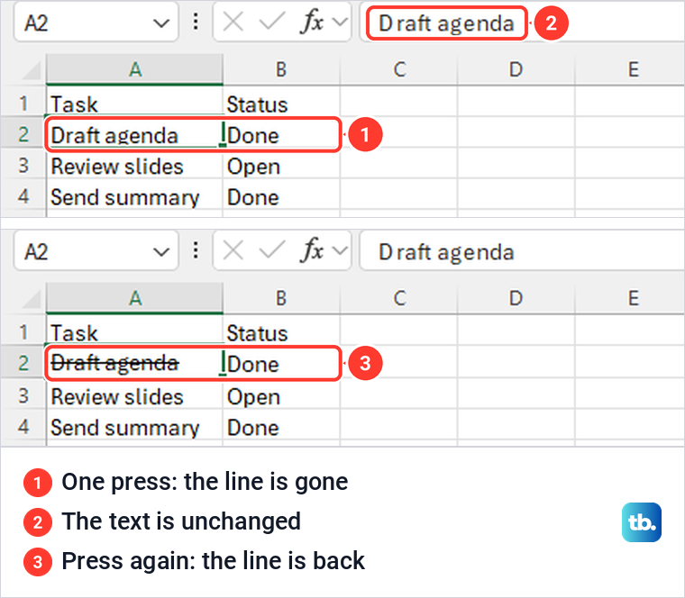
In Excel for Windows, click the cell, or drag over a range, and press Ctrl + 5. On our task list, A2 held Draft agenda with a line through it. One press removed the line and a second press put it back, while the formula bar showed Draft agenda the whole time.
That is the point of strikethrough. You cross out text to show a job is finished, not to delete it, so the cell keeps its value and stays readable. Microsoft's shortcut list describes the keys as Apply or remove strikethrough formatting, which is why the same press works both ways.
A range works the same way. We selected A11 and A12, which held Call vendor and File notes, pressed the keys once, and both cells were crossed out together. If you like working from the keyboard, our list of Excel keyboard shortcuts worth learning has the other formatting keys that sit next to this one.
Find Strikethrough in the Format Cells box
If you prefer menus, open the Home tab and click the small arrow in the bottom right corner of the Font group. Its ScreenTip on our PC read Font Settings (Ctrl+Shift+F) and said you can add visual effects such as strikethrough and superscript. Microsoft calls this arrow the Dialog Box Launcher.
The launcher opened Format Cells straight on the Font tab. Under Effects there are three boxes, Strikethrough, Superscript and Subscript. Tick Strikethrough, check that the Preview shows the line, and click OK. On our sheet only the selected cell, A2, was crossed out.
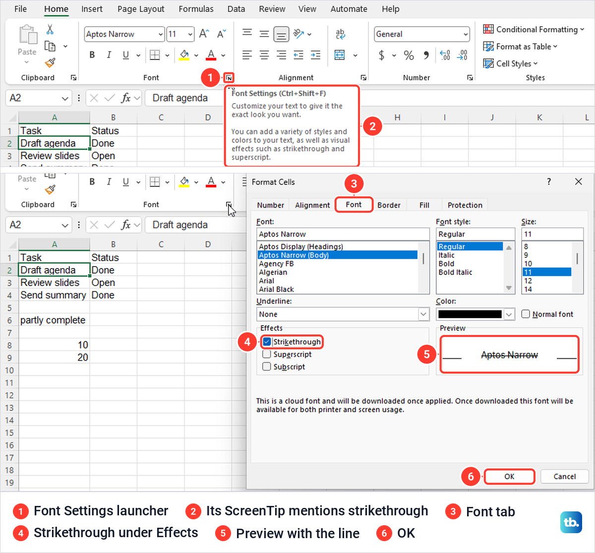
You can reach the same box with Ctrl + 1, which Microsoft lists for opening Format Cells, or by right-clicking the cell and choosing Format Cells. The right-click menu on our PC had no Strikethrough item of its own, and neither did the small formatting toolbar that appears above it. We used that route on A3, Review slides, and only A3 gained the line while its status stayed Open.
With the default Aptos Narrow font, ticking Strikethrough also changed a note at the bottom of the box to say this is a cloud font that will be downloaded once applied. The note only says Excel will download the font. There is nothing to click, and the line appeared as soon as we clicked OK.
Cross out only one word in a cell
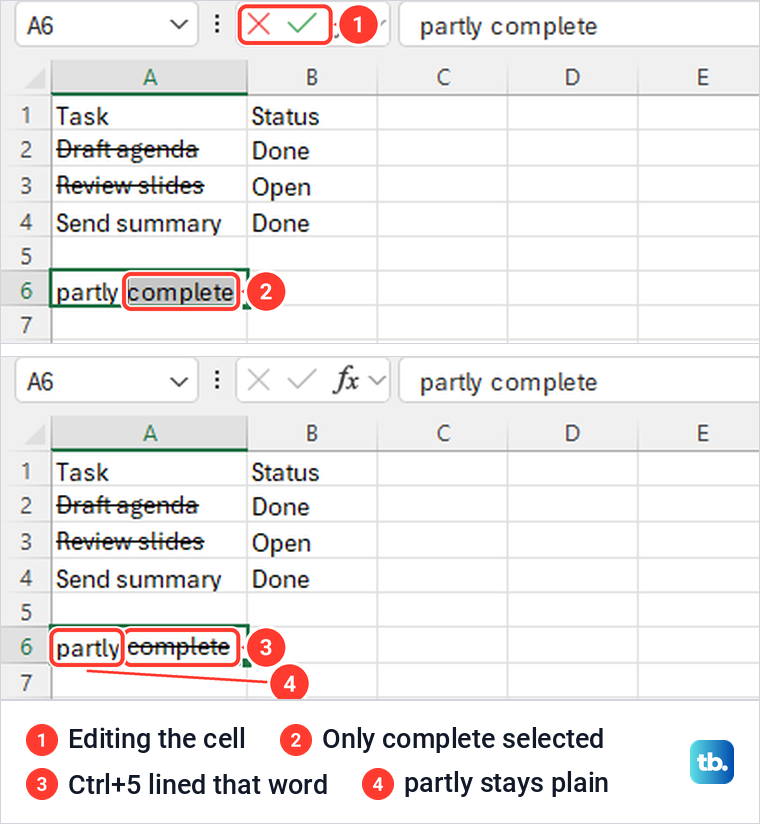
A line can cover part of a cell, which is handy for a note such as partly complete. Click the cell and press F2 to edit it, or double-click it as Microsoft suggests for selecting part of a cell's text. Then select only the characters you want crossed out, press Ctrl + 5 and press Enter.
On our sheet, A6 held partly complete. We selected only the word complete while editing, pressed the keys, and after Enter the cell showed partly in plain text and complete crossed out. While the cell was being edited, Excel greyed out the Number, Styles and Cells groups, but the Font group stayed available.
Cross out tasks automatically when they are Done
For a to-do list, you can let Excel draw the line for you. A conditional formatting rule watches a status column and crosses out the task when its status says Done, then removes the line if the status changes back. Our list had tasks in A2 to A4 and Done or Open beside each one in column B.
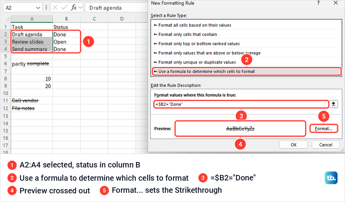
Select the task names, A2 to A4 on our sheet, but not the status column. Open Home > Conditional Formatting > New Rule and choose Use a formula to determine which cells to format. In the box labelled Format values where this formula is true, type =$B2="Done".
The dollar sign keeps the rule looking at column B, while the 2 without a dollar sign lets each row check its own status. Microsoft's rule for these formulas is that they must return True or False, and this one does. Write the row number of the first selected cell, so A2 to A4 starts with B2.
Click Format. The box that opens is a shorter Format Cells with only Number, Font, Border and Fill tabs, and on our PC its Strikethrough box started half filled rather than empty. Click it until it shows a tick, then click OK. The rule's Preview showed AaBbCcYyZz crossed out, and a final OK saved the rule.
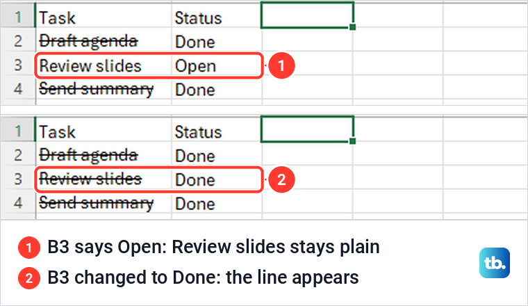
Draft agenda and Send summary, both marked Done, were crossed out at once. Review slides stayed plain while B3 said Open. When we changed B3 to Done, Review slides gained the line, and changing it back to Open took the line away again.
The rule compares text, so the status has to be typed the same way every time. An Excel drop-down list for Done and Open in column B takes care of that.
Fix a rule that misses some rows
If some rows marked Done stay plain, check the range the rule covers. Open Conditional Formatting > Manage Rules and first look at the Show formatting rules for list at the top. Ours read Current Selection, which lists only the rules for the cells you selected, so pick the worksheet there as Microsoft advises, then find the rule and read its Applies to box.
To see what a wrong range does, we narrowed Applies to from =$A$2:$A$4 to =$A$2 and clicked OK. Send summary in A4 lost its line even though B4 still said Done. Typing =$A$2:$A$4 back into the same box brought the line back.
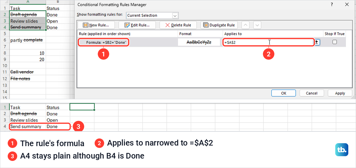
To remove only this rule, select it in the same Rules Manager and click Delete Rule, or in Excel for the web use the delete icon on that rule, as Microsoft describes. Clear Rules on the Conditional Formatting menu is broader, because Clear Rules from Selected Cells and Clear Rules from Entire Sheet remove every rule in that scope. If other rules on the sheet also misbehave, our guide to fix conditional formatting in Excel works through the other causes.
Remove strikethrough without losing other formatting
The cleanest way to remove a line you added is the way you added it. Select the cell and press Ctrl + 5, or open Format Cells and clear the Strikethrough box. Both change only the line, unlike Clear Formats below.
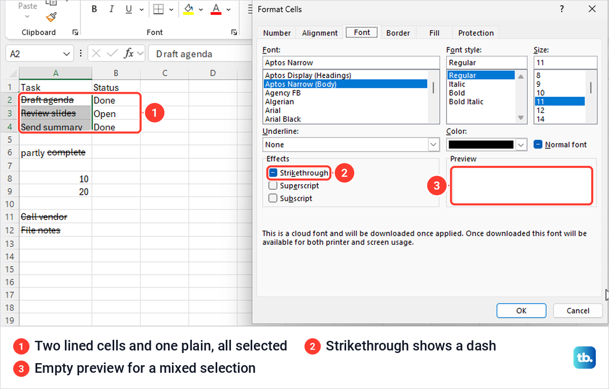
A selection that mixes crossed-out and plain cells needs one extra click. When we selected two lined cells and one plain cell and opened Format Cells, the Strikethrough box showed a dash instead of a tick or an empty box. Pressing Alt + K, the box's access key, ticked it, and pressing it again cleared it, so keep going until the box is empty before you click OK.
Clear Formats is the bigger hammer. Microsoft's steps on the desktop are Home > Editing > Clear > Clear Formats, and it takes the other formatting off those cells as well, not just the line. In Excel for the web we used the same Clear menu on A12, and the crossed-out File notes went back to plain text.
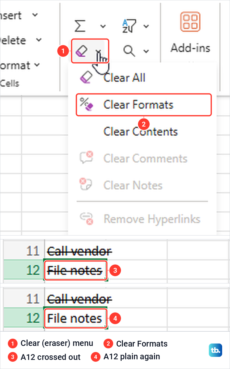
Before you clear the formats on a large, carefully styled sheet, make a copy of the Excel file so you can compare the two afterwards. If the line comes from a conditional rule, edit or delete the rule instead, as in the section above. If the cells sit in a formatted Excel table and the styling comes from the table itself, follow the steps to clear Excel table formatting.
Use strikethrough in Excel for the web
Excel for the web had a Strikethrough button on its Home tab, which the desktop ribbon on our PC did not. Open the workbook in Editing mode, select the cells, and on the Home tab click Strikethrough in the Font group, the crossed-out ab icon. One click crossed out A11 on our sheet and a second click removed the line.
The Font group in the browser had no Font Settings launcher. Pressing Ctrl + 1 in Edge opened a side pane called All formatting options, with Number, Alignment, Font and Border tabs. On its Font tab, the Strikethrough button under Effects crossed out A12 the moment we clicked it, with no OK button to press.
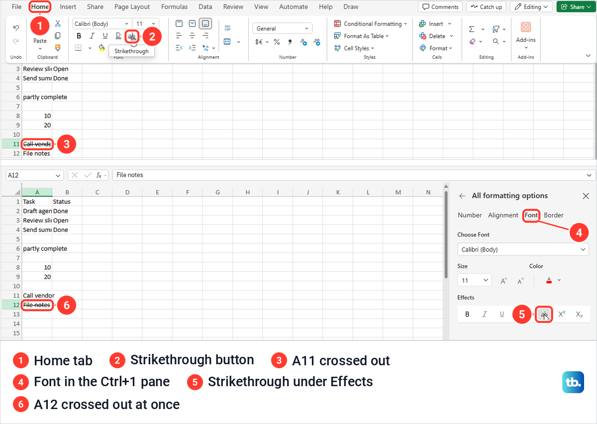
Microsoft's help page for this still describes a Font Settings button that opens a Format Cells dialog, so do not be surprised if you cannot find it. On our screen, Ctrl + 1 opened the full font options in a pane instead. If you have not opened a workbook in a browser before, our Excel guide for beginners has a section on using Excel in a browser.
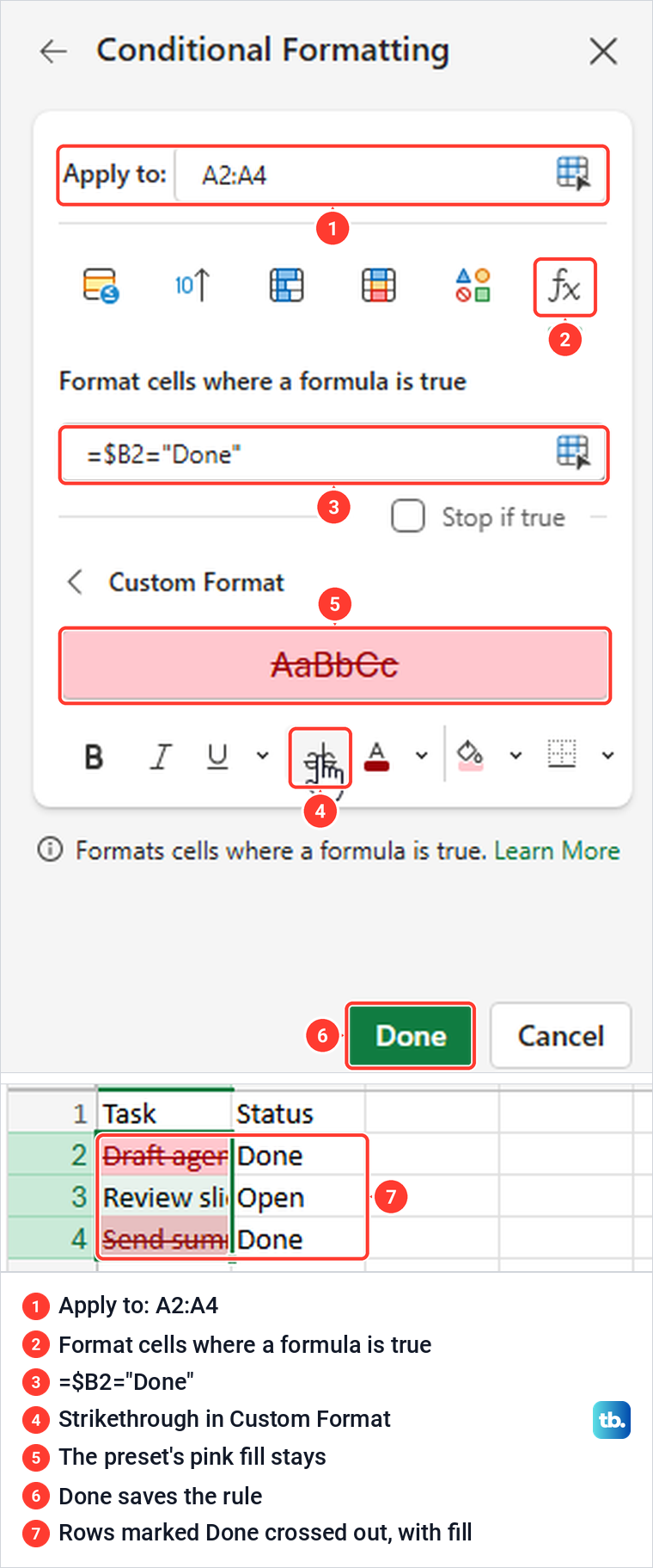
The Done rule works in the browser too, with different labels. Select the tasks, open Conditional Formatting > Manage Rules and click New Rule. Pick the fx icon, Format cells where a formula is true, type =$B2="Done", then under Format Style click the plus sign to open Custom Format and click its Strikethrough button. Click Done to save the rule.
The custom format starts from the first preset, a pink fill with dark red text. We left those as they were, so our Done rows came out crossed out and shaded pink, and A3 followed B3 as it changed between Done and Open. The fill and font colour buttons sit in the same row as Strikethrough if you want the line alone.
When the formatting buttons are greyed out
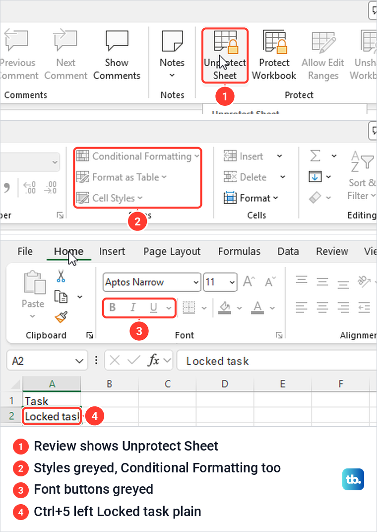
A protected sheet can block strikethrough when its Format cells permission is off. We protected a sheet with Review > Protect Sheet, where the Format cells permission is unticked by default. On that sheet Ctrl + 5 and Ctrl + 1 did nothing at all, with no message, and the Font buttons and Conditional Formatting were greyed out on the Home tab.
The giveaway is on the Review tab, where the button reads Unprotect Sheet instead of Protect Sheet. After we clicked Unprotect Sheet, Ctrl + 5 crossed out the cell straight away. If the owner set a password and you have permission to edit, unprotect the Excel worksheet with it first.
If you protect a list yourself and still want people to cross out tasks, tick Format cells in the Protect Sheet box. Microsoft says that option lets people change any of the options in the Format Cells or Conditional Formatting dialog boxes. Our guide to lock cells in Excel explains which cells stay editable once protection is on.
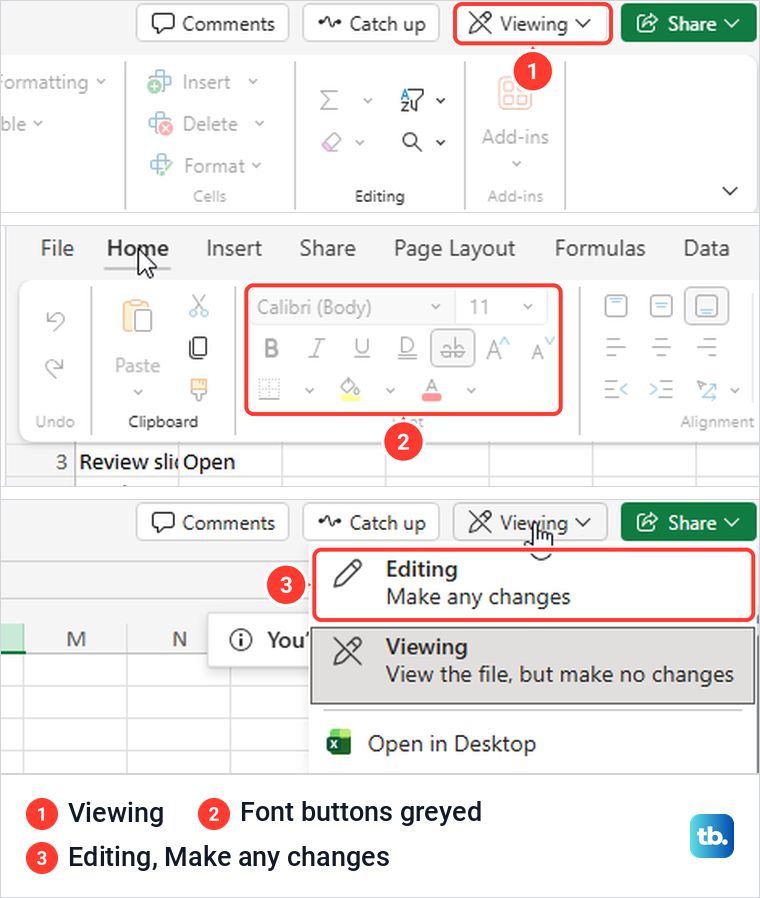
In Excel for the web, greyed buttons can mean the workbook is open in Viewing mode. With Viewing on, the whole Home ribbon was grey on our screen, Strikethrough included. Open the Viewing menu at the top right, choose Editing, and the button worked again.
Why a formula result looks crossed out
In Excel for Microsoft 365, Excel can draw the line by itself. Microsoft says that in Partial and Manual calculation, Excel denotes a stale cell with a strikethrough to show that its value is out of date. It looks like the font effect, but it is a warning that the result is out of date, and recalculating clears it.
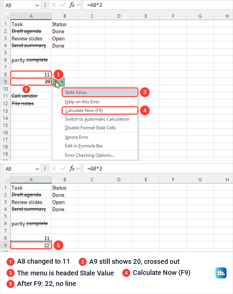
We reproduced it on purpose. With Formulas > Calculation Options set to Manual, the Format Stale Values option in the same menu was ticked. We changed A8 from 10 to 11, and A9, which holds =A8*2, kept showing 20 with a line through it and a green triangle in the corner. The status bar showed the word Calculate.
The warning button beside the cell said the value in this cell is stale and to calculate the workbook to see an up-to-date value. Its menu, headed Stale Value, offered Calculate Now (F9), Switch to Automatic Calculation and Disable Format Stale Cells. Pressing F9 changed A9 to 22 and the line disappeared.
Do not switch off Format Stale Values to make the line go away. Microsoft warns that doing so will not cause the values to be updated, and it recommends keeping the option on. To stop seeing stale results at all, set Calculation Options back to Automatic. If a formula still shows the wrong answer after F9, our guide to fix Excel formulas that are not working covers the next checks.
Strikethrough shortcut on a Mac
Microsoft's shortcut list for Excel for Mac gives Shift + Cmd + X to apply or remove strikethrough formatting. It also lists Cmd + 1 for the Format Cells dialog.
How we tested this guide
We tested this in Excel for Microsoft 365 on Windows 11, version 25H2, and in Excel for the web in Microsoft Edge, crossing out tasks on a practice list.
Frequently Asked Questions
What is the shortcut for strikethrough in Excel?
On Windows it is Ctrl + 5, and the same keys remove the line. Microsoft lists Shift + Cmd + X for Excel for Mac.
How do I cross out only one word in a cell?
On Windows, press F2 to edit the cell, select the word, press Ctrl + 5 and then Enter. On our sheet only the selected word was crossed out and the rest of the cell stayed plain.
Can Excel cross out a task when I mark it Done?
Yes. A conditional formatting rule with the formula =$B2="Done" and Strikethrough as its format crossed out each task whose status in column B said Done. The line came and went as we changed the status.
Where is Strikethrough in Excel for the web?
It is a button in the Font group on the Home tab, available in Editing mode. Ctrl + 1 also opens an All formatting options pane with Strikethrough on its Font tab.
Why did Excel cross out a formula result on its own?
In Excel for Microsoft 365, the result is probably stale because the workbook is in Manual or Partial calculation. Press F9 to recalculate, which removed the line on our sheet, or set Calculation Options back to Automatic.
Why will Excel not let me apply the line?
On the desktop, the sheet is probably protected without the Format cells permission, and Review then shows Unprotect Sheet. In Excel for the web, check that the workbook is in Editing mode rather than Viewing.
How do I remove a line that keeps coming back?
A conditional formatting rule is probably drawing it. Open Conditional Formatting > Manage Rules, then edit the rule, narrow its Applies to range or select it and click Delete Rule.