
To calculate standard deviation in Excel, click an empty cell, type =STDEV.S(A2:A9) if your numbers are a sample, or =STDEV.P(A2:A9) if they are the whole population, and press Enter. Change A2:A9 to the cells that hold your numbers. On our sheet of eight made-up scores, the sample formula returned 2.13809 and the population formula returned exactly 2.
The two answers differ because the sample formula divides the squared distances from the average by one less than the number of values, which Microsoft calls the "n-1" method, while the population formula divides them by the full count. Use STDEV.S when your rows are a sample taken from a bigger group, and STDEV.P when they are every member of the group you want to describe.
The short version
- Sample: type
=STDEV.S(A2:A9)and press Enter. - Whole population: type
=STDEV.P(A2:A9)instead. - One answer per group: use a PivotTable and set its value summary to StdDev or StdDevp.
- Text and TRUE: both formulas skip them in a range, while STDEVA is the version that can count them.
- #DIV/0!: STDEV.S needs at least two numbers in the range.
Which standard deviation formula to use
| What you need | Use this | What it counts |
|---|---|---|
| The spread of a sample | =STDEV.S(A2:A9) | Squared distances from the average, divided by one less than the count, then the square root. 2.13809 on our scores |
| The spread of a whole population | =STDEV.P(A2:A9) | Squared distances from the average, divided by the full count, then the square root. 2 on our scores |
| A sample where TRUE and text should count | =STDEVA(D2:D5) | TRUE as 1 and the word note as 0 on our sheet, giving 3.593976 |
| A whole population where TRUE and text should count | STDEVPA | Microsoft's population version of STDEVA |
| One result for each group | A PivotTable set to StdDev or StdDevp | One value per row label, plus a Grand Total |
| Only the rows a filter shows | SUBTOTAL with function number 7 or 8 | Sample (7) or population (8) of the visible rows, per Microsoft |
Older workbooks may use STDEV and STDEVP. Microsoft lists STDEV as the earlier name of STDEV.S and keeps STDEVP among its compatibility functions, and it says renamed functions remain available with their old name, so those formulas still work. For a new formula, type STDEV.S or STDEV.P.
Calculate a sample standard deviation with STDEV.S
Put your numbers in one column with a heading above them. Our example has eight scores in A2:A9 and a North or South label beside each one in column B. If you are new to typing data into a sheet, our Excel basics for beginners guide shows how to start a blank workbook and type values into cells.
Click an empty cell for the answer, type =STDEV.S( and drag over the numbers, or type the range yourself. As soon as we typed A2:A9, Excel drew a blue outline around those cells and showed a ScreenTip under the cell reading "STDEV.S(number1, [number2], ...)".
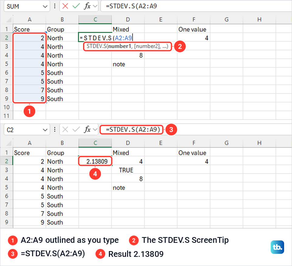
Type the closing bracket and press Enter. Our cell showed 2.13809 and the formula bar showed =STDEV.S(A2:A9). That is five decimal places at the default column width, and the full value, 2.138089935, appears in the Function Arguments box further down this guide.
The range does not have to be one block. Excel's own help line says the function takes 1 to 255 numbers or references that contain numbers, so you can list separate ranges or single cells with commas between them.
Calculate a population standard deviation with STDEV.P
Type =STDEV.P(A2:A9) in another empty cell and press Enter. Our same eight scores returned exactly 2, against 2.13809 for the sample formula, because the population formula divides the squared distances by 8 where the sample formula divides them by 7.
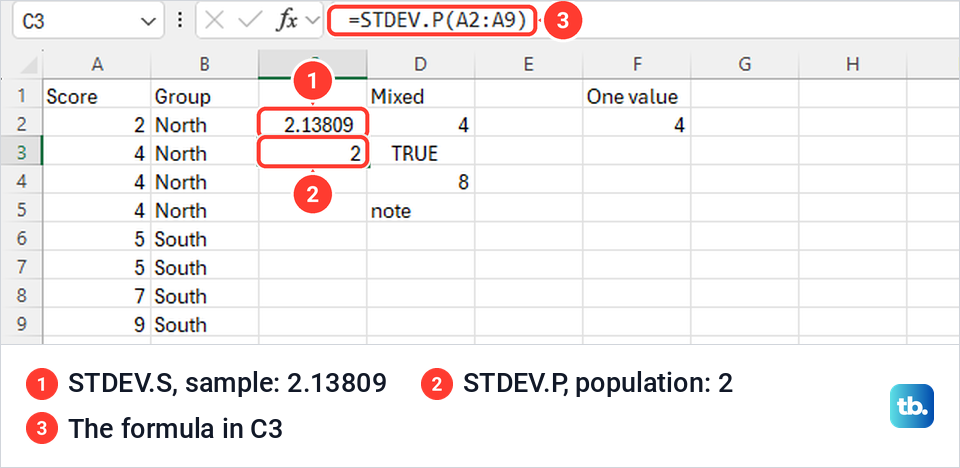
For the same numbers, the population answer is never larger than the sample answer. Microsoft notes that for large sample sizes, STDEV.S and STDEV.P return approximately equal values, while with our eight scores the difference is easy to see.
Microsoft describes standard deviation as a measure of how widely values are dispersed from the average value. If you need the squared version of that spread, see how to calculate variance with Excel, which uses the same sample and population pairing.
Check the answer by hand
If your own answer does not match Excel's, check the divisor first. Our eight scores, 2, 4, 4, 4, 5, 5, 7 and 9, average 5. Their distances from 5 are 3, 1, 1, 1, 0, 0, 2 and 4, and those distances squared add up to 32.
Divide 32 by 7, one less than the count, and take the square root, and you get 2.13809, the STDEV.S answer. Divide 32 by 8 instead and the square root is exactly 2, the STDEV.P answer. If your hand result matches the other formula, you used the other divisor, and if it matches neither, compare which cells each of you counted.
Use Insert Function instead of typing
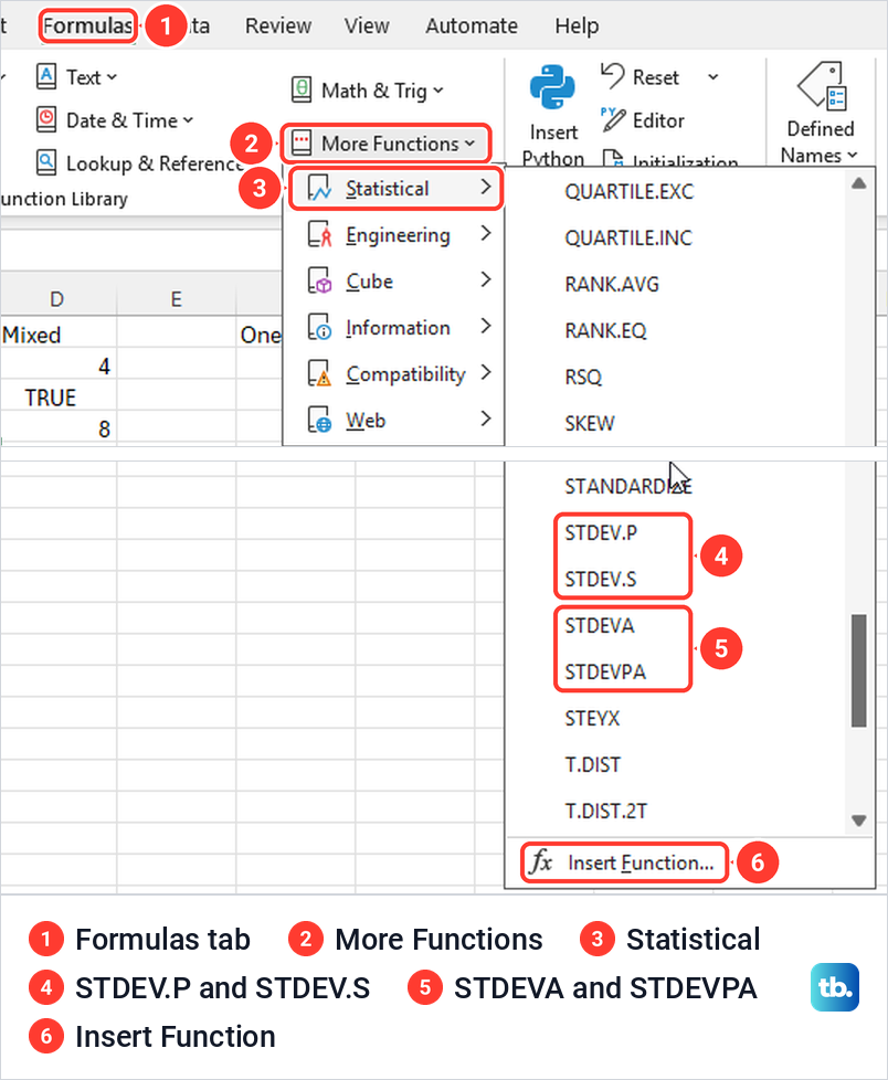
If you would rather pick the function from a list, click the answer cell and open Formulas > More Functions > Statistical. The list is long and alphabetical, so scroll past STANDARDIZE to reach STDEV.P, STDEV.S, STDEVA and STDEVPA.
Choosing STDEV.S opened the Function Arguments box. Its help line read "Estimates standard deviation based on a sample (ignores logical values and text in the sample)." With A2:A9 in Number1, it showed "Formula result = 2.138089935" before we clicked OK, and OK put 2.13809 in the cell.
Pressing Shift + F3 opens the Insert Function dialog straight from the sheet. Type STDEV.P under Search for a function, select Go, and its description reads "Calculates standard deviation based on the entire population given as arguments." Our list of useful Excel keyboard shortcuts has more like it.
Check Number1 before you click OK. When we opened STDEV.P in C5, under three results already in C2:C4, Excel filled Number1 with C2:C4 by itself and previewed 0.06509622, the spread of our earlier answers rather than of the scores. Replace the whole contents of the box with A2:A9, and the preview changes, to 2 on our sheet.
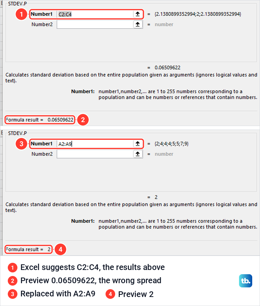
It does not happen every time. STDEV.S chosen from the ribbon in C4, under two results, opened with an empty Number1 box, so read the box each time rather than trusting it.
Find the standard deviation for each group with a PivotTable
When your data has a label column, such as region, class or product, a PivotTable gives one standard deviation per label. First create a PivotTable in Excel from the data, with the label field in Rows and the number field in Values.
Ours started as Sum of Score, with 14 for North, 26 for South and a Grand Total of 40, because a PivotTable sums numbers by default. Right-click any value, choose Value Field Settings, and scroll the Summarize value field by list to StdDev for a sample or StdDevp for a whole population, then select OK.
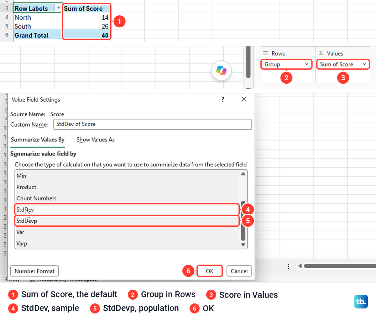
With StdDev, North showed 1, South 1.914854216 and the Grand Total 2.138089935, the same as STDEV.S on all eight scores. StdDevp gave 0.866025404, 1.658312395 and 2.
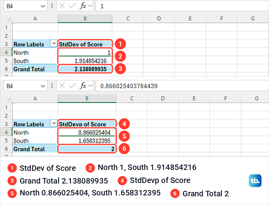
The column heading changes to StdDev of Score or StdDevp of Score, and you can rename it in the Custom Name box of the same dialog. The PivotTable showed nine decimal places where our formula cells showed five, so format the column if you want fewer.
Calculate standard deviation for filtered rows only
For the spread of only the rows a filter leaves on screen, Microsoft's SUBTOTAL function takes a function number first and the range second. Function number 7 gives the sample standard deviation and 8 the population one, and Microsoft says filtered-out cells are always excluded. Click an empty cell outside the list and type an equals sign, SUBTOTAL and an opening bracket, then 7 or 8, a comma, your number range and a closing bracket, and press Enter.
Microsoft's table pairs 7 and 107 with STDEV, and 8 and 108 with STDEVP. Function numbers 107 and 108 also leave out rows you hide by hand, the way our guide to hide rows in Excel describes, while 7 and 8 keep those rows in the result.
Microsoft adds that SUBTOTAL is designed for columns of data, or vertical ranges, so keep the numbers in one column. If the filtered view is not showing the rows you expect, fix filters that are not working before trusting the result.
If the range may hold error cells, Microsoft's AGGREGATE function is the other route. Its table lists function number 7 for STDEV.S and 8 for STDEV.P, with option 6 to ignore error values and option 7 to ignore hidden rows and error values together. Type an equals sign, AGGREGATE and an opening bracket, then 7 or 8, a comma, 6, a comma, your range and a closing bracket, and press Enter.
Decide whether text and TRUE values should count
STDEV.S and STDEV.P only use the numbers in a range. Microsoft's help says that for a reference, only numbers in that array or reference are counted, while TRUE, FALSE and numbers written as text count when you type them straight into the formula instead of referring to cells.
Our Mixed column held 4, the logical value TRUE, 8 and the word note. =STDEV.S(D2:D5) returned 2.828427, the standard deviation of 4 and 8 alone. =STDEVA(D2:D5) returned 3.593976, which is the sample standard deviation of 4, 1, 8 and 0, so on our sheet it counted TRUE as 1 and the text note as 0.
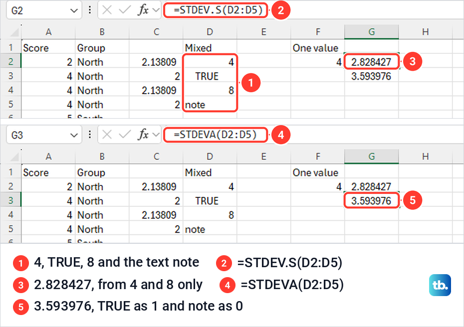
Use STDEVA only when TRUE, FALSE or text entries really belong in the data, such as yes or no answers stored as TRUE and FALSE. Microsoft's STDEVA page says TRUE counts as 1 and text or FALSE as 0, and STDEVPA is the population version for the same kind of data.
Turn on the Analysis ToolPak
Excel's Analysis ToolPak can build a Descriptive Statistics report that, in Microsoft's words, gives information about the central tendency and variability of your data. Microsoft says to open it from Data Analysis on the Data tab, and to load the add-in if that command is not there.
On our PC the Data tab had no Data Analysis button. Under File > Options > Add-ins, Excel listed Analysis ToolPak among the Inactive Application Add-ins, so it was installed but switched off.
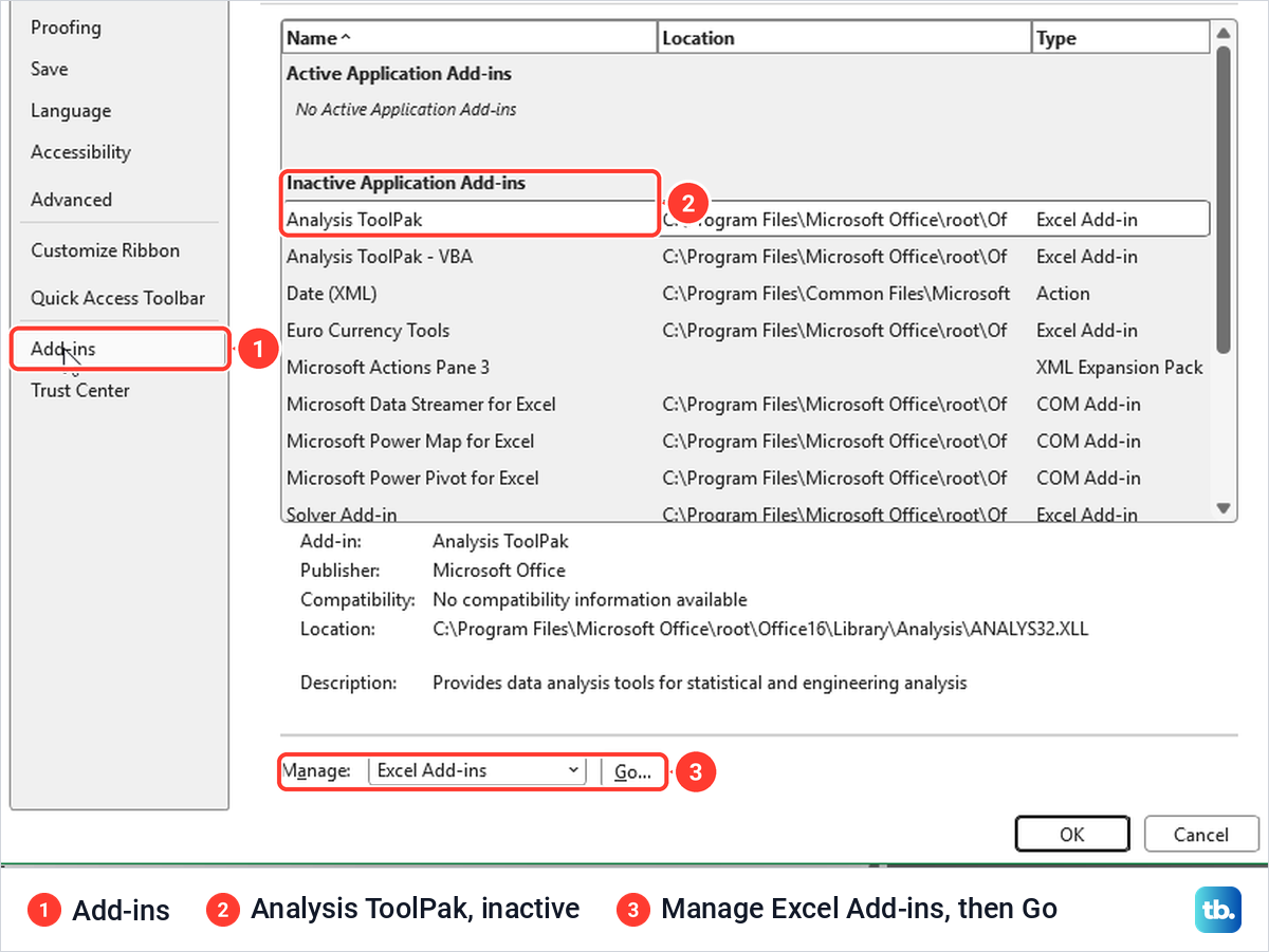
Microsoft's steps to switch it on are to choose Excel Add-ins in the Manage box on that page, select Go, tick Analysis ToolPak and select OK. Our Add-ins box listed it unticked, alongside Analysis ToolPak - VBA, Euro Currency Tools and Solver Add-in. For a single standard deviation, the formulas above are quicker.
Calculate standard deviation in Excel for the web
The same two formulas work in a browser. In Excel for the web in Microsoft Edge, =STDEV.S(A2:A9) returned 2.13809 and =STDEV.P(A2:A9) returned 2 on a copy of our scores, matching the desktop app.
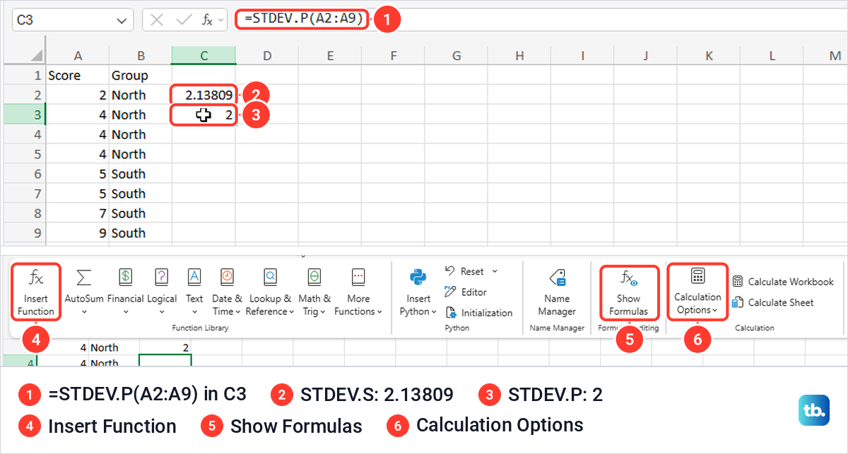
The web Formulas tab has labelled Insert Function, Show Formulas and Calculation Options buttons, while on our desktop Show Formulas was a small unlabelled icon. Microsoft's STDEV.S and STDEV.P pages also list Excel for Mac among the versions they apply to.
Fix a #DIV/0! error or a number that looks wrong
STDEV.S needs at least two numbers, because it divides the squared distances by one less than the count, which is zero for a single number. With a single value in F2, =STDEV.S(F2:F2) showed #DIV/0! on our sheet, while =STDEV.P(F2:F2) returned 0.
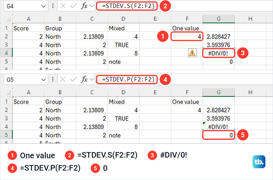
So when STDEV.S shows #DIV/0!, count the numbers the range really holds. Text, TRUE and empty cells in a range are not counted, so a column of numbers stored as text can leave too few.
If the answer is a number but not the one you expect, check that the range covers every row, that you picked the right one of STDEV.S and STDEV.P, and that no number is stored as text. While you edit a formula, Excel outlines the range it uses, as in our first screenshot, which makes a range that stops short easy to spot.
Fix a formula that shows as text
If the cell shows =STDEV.S(A2:A9) instead of a number, the cell was probably formatted as Text before you typed. That is what we saw after setting a cell to Text, where the formula sat in the cell as plain text.
Changing the format back to General was not enough on its own. The formula stayed as text until we clicked the cell, pressed F2 and then Enter, which is the order Microsoft gives, and then it returned 2.13809.
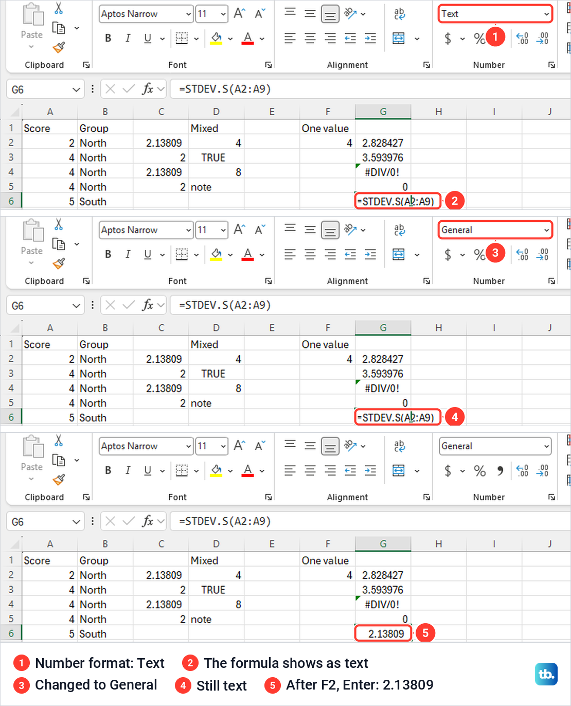
Show Formulas can look like the same problem, except that every formula on the sheet shows its text at once. Press Ctrl + ` or select the Show Formulas icon in the Formula Auditing group of the Formulas tab to switch it off. For other causes, our guide to fix formulas showing as text goes through them one by one.
Fix a result that does not update
A standard deviation that stays the same after you change a score can mean the workbook is set to manual calculation. Check File > Options > Formulas, where Workbook Calculation offered Automatic, Partial and Manual on our PC. Microsoft calls Automatic the default calculation setting.
With Manual selected, we changed the first score from 2 to 3. The results did not change, Excel drew them struck through with green triangles, and the status bar read Calculate. Switching back to Automatic recalculated them at once, and C2 showed 1.95941.
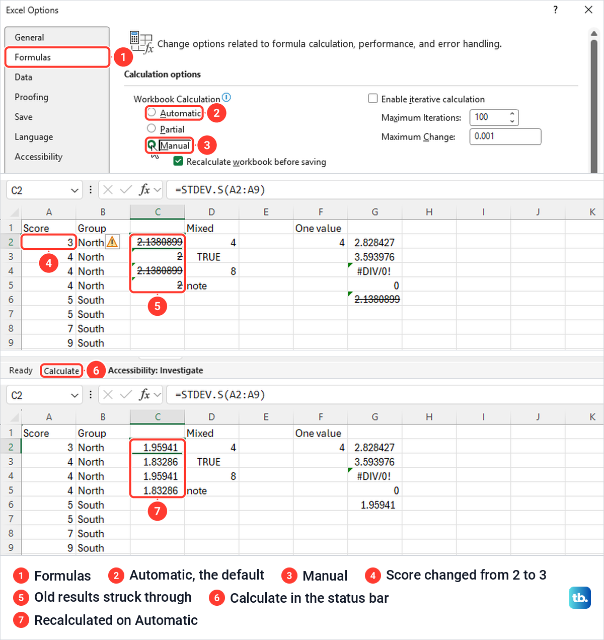
Microsoft notes that in the desktop app this option affects all open workbooks, and that on Manual you recalculate by pressing F9. For calculation problems beyond this one, work through our guide to fix Excel formulas that are not working.
Fix a sheet that will not let you type
If Excel will not let you type the formula at all, the sheet may be protected. On our protected sheet, Excel said "The cell or chart you're trying to change is on a protected sheet," and the formula went in after Review > Unprotect Sheet. If you have permission to edit, unprotect an Excel worksheet first, or ask whoever set it up for the password.
How we tested this guide
We tested this in Excel for Microsoft 365 on Windows 11, version 25H2, running STDEV.S and STDEV.P on a sheet of eight made-up scores.
Frequently Asked Questions
What is the formula for standard deviation in Excel?
Type =STDEV.S(A2:A9) for a sample or =STDEV.P(A2:A9) for a whole population, replacing A2:A9 with your own cells, and press Enter. On our eight scores in A2:A9 they returned 2.13809 and 2.
Should I use STDEV.S or STDEV.P?
Use STDEV.S when your rows are a sample from a bigger group and STDEV.P when they are the whole group. The sample version divides the squared distances by one less than the count, so for the same numbers it never gives the smaller answer.
Why is my Excel standard deviation different from my manual answer?
Check the divisor first, since STDEV.S divides the squared distances by one less than the count and STDEV.P by the full count. Then check that both use the same numbers, because both formulas skip text and TRUE in a range.
How do I calculate standard deviation by group?
Build a PivotTable with the group in Rows and the numbers in Values, then change Value Field Settings from Sum to StdDev or StdDevp. Ours gave one result per group plus a Grand Total.
Why does STDEV.S show #DIV/0!?
The range holds fewer than two numbers. One number gave #DIV/0! with STDEV.S on our sheet, while STDEV.P returned 0 for the same cell.
How can I calculate standard deviation for visible rows only?
Microsoft's SUBTOTAL function with function number 7 (sample) or 8 (population) skips rows a filter hides. Use 107 or 108 to leave out rows you hid by hand as well.
Can I still use STDEV in an older workbook?
Yes. Microsoft keeps STDEV and STDEVP for compatibility, so old formulas still work, but it recommends the renamed STDEV.S and STDEV.P for new ones.